The SSM Procedure

This example describes how you can include components in your model that follow a transfer function model. Transfer function models, a generalization of distributed lag models, are useful for capturing the contributions from lagged values of the predictor series. Box and Jenkins popularized ARIMA models with transfer function inputs in their famous book (Box and Jenkins, 1976). This example shows how you can specify an ARIMA model that is suggested in that book to analyze the data collected in an experiment at a chemical factory. The data set, called Series J by Box and Jenkins, contains sequentially recorded measurements of two variables: x, the input gas rate, and y, the output CO. For the output CO, Box and Jenkins suggest the model

where is the intercept, is a zero-mean noise term that follows a second-order autoregressive model (that is, ), and follows a transfer function model

The model for is specified by using the ratio of two polynomials in the backshift operator . Alternatively, this model can also be described as follows:

In this alternate form, it is easy to see that the equation for can also be seen as a state evolution equation for a one-dimensional state with a () transition matrix and state regression variables , and (lagged values of x). This state equation has no disturbance term.

The following statements define the data set Seriesj. The variables x3, x4, and x5, which denote the appropriately lagged values of x, are also created. These variables are used later in the STATE statement that is used to specify .

data Seriesj;
   input x y @@;
   label x = 'Input Gas Rate'
         y = 'Output CO2';
   x3 = lag3(x);
   x4 = lag4(x);
   x5 = lag5(x);
   obsIndex = _n_;
   label obsIndex = 'Observation Index';
datalines;
-0.109  53.8  0.000  53.6  0.178  53.5  0.339  53.5
 0.373  53.4  0.441  53.1  0.461  52.7  0.348  52.4
 0.127  52.2 -0.180  52.0 -0.588  52.0 -1.055  52.4

   ... more lines ...   

The following SSM procedure statements carry out the modeling of y, the output CO, according to the preceding model:

 proc ssm data=Seriesj(firstobs=6);
     id obsIndex;
     parms delta /lower=-0.9999 upper=0.9999;
     state tfstate(1) T(g)=(delta) W(g)=(x3 x4 x5) a1(1) checkbreak;
     comp tfinput = tfstate[1];
     trend ar2(arma(p=2)) ;
     intercept = 1;
     model y = intercept tfinput ar2 ;
     eval modelCurve = intercept + tfinput;
     forecast out=For;
 run;

The coefficient of the denominator polynomial, , is specified in a PARMS statement. It is constrained to be less than 1 in magnitude, which ensures that the transfer function term does not have explosive growth. The transfer function model for is specified in a STATE statement that defines a one-dimensional state named tfstate. In this statement, the transition matrix (which contains only one element, ) is specified by using the T(g)= option; the state regression variables x3, x4, and x5 are specified by using the W(g)= option; and the CHECKBREAK option is used to turn on the search for unexpected changes in the behavior of . The COV option is absent from this STATE statement because the disturbance term is absent from the state equation for . Moreover, because nothing can be assumed about the initial condition of this state equation, it is taken to be diffuse (as signified by the A1 option). Note that the first five observations of the input data set, Seriesj, are excluded from the analysis to ensure that the state regression variables x3, x4, and x5 do not contain any missing values. The component that is associated with tfstate, named tfinput, is specified in a COMPONENT statement that follows the STATE statement. A zero-mean, second-order autoregressive noise term, named ar2, is specified by using a TREND statement. Next, a constant regression variable, intercept, is defined to be used in the MODEL statement to capture the intercept term . Finally, the model specification is completed by specifying the response variable, y, and the three right-hand terms in the MODEL statement. Next, an EVAL statement is used to specify a component, modelCurve, which is the sum of the intercept and the transfer function input (). The modelCurve component represents the structural part of the model and is defined only for output purposes: its estimate is output (along with the estimates of other components) to the data set that is specified in the OUT= option of the OUTPUT statement.

Note that the modeling of output CO according to this model is also illustrated in Example 7.3 of the PROC ARIMA documentation (see Chapter 7: The ARIMA Procedure). The ARIMA procedure handles the computation of the transfer function slightly differently than the way it is estimated by the SSM procedure. However, despite this algorithmic difference in the modeling procedures, for this example the estimated parameters agree quite closely (barring the sign conventions that are used to specify the model parameters).

Output 27.10.1 shows the estimate of , the intercept in the model. Output 27.10.2 shows the estimate of , the coefficient in the denominator polynomial of the transfer function. Output 27.10.3 shows the regression estimates of the state regression variables x3, x4, and x5 (which correspond to the coefficients of the numerator polynomial). Output 27.10.4 shows the estimates of the parameters of the AR(2) noise term.

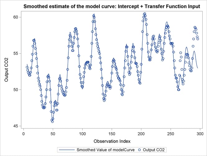
The following statements produce a time series plot of the estimate of modelCurve—that is, the estimate of the structural part of the model ()—along with the scatter plot of the observed values of the output CO. The plot, shown in Output 27.10.5, seems to indicate that the model captures the relationship between the input gas rate and the output CO quite well, at least up to the observation index 250.

 proc sgplot data=For;
    title "Smoothed estimate of the model curve: Intercept + Transfer Function Input";
    series x=obsIndex y=smoothed_modelCurve;
    scatter x=obsIndex y=y;
 run;

Output 27.10.5: Smoothed Estimate of

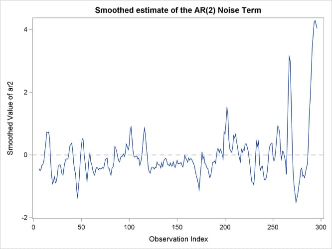
The plot shown in Output 27.10.6 shows the estimate of the noise term, ar2, which is produced by the following statements:

 proc sgplot data=For;
    title "Smoothed estimate of the AR(2) Noise Term";
    series x=obsIndex y=smoothed_ar2;
    refline 0 / axis=y lineattrs=GraphReference(pattern = Dash);
 run;

If you compare the scales of these two plots, it appears that the noise term is relatively small and that most of the variation in output CO can be explained by the structural part of the model. It does, however, appear that the model fit deteriorates toward the latter part of the sample. The structural break analysis summary, shown in Output 27.10.7, indicates strong evidence of structural break in the behavior of at or near the observation index 264. Obviously, this type of structural break analysis can be quite useful in industrial quality-control applications.

Output 27.10.6: Smoothed Estimate of the AR(2) Noise Term