The SSM Procedure
-
Overview

- Getting Started
-
Syntax
-
DetailsState Space Model and NotationTypes of Sequence DataOverview of Model Specification SyntaxFiltering, Smoothing, Likelihood, and Structural Break DetectionEstimation of User-Specified Linear Combination of State ElementsContrasting PROC SSM with Other SAS Procedures Predefined Trend ModelsPredefined Structural ModelsCovariance ParameterizationMissing ValuesComputational IssuesDisplayed OutputODS Table NamesODS Graph NamesOUT= Data Set
-
ExamplesBivariate Basic Structural Model Panel Data: Random-Effects and Autoregressive ModelsBackcasting, Forecasting, and InterpolationLongitudinal Data: Smoothing of Repeated MeasuresA User-Defined Trend ModelModel with Multiple ARIMA ComponentsDynamic Factor ModelingDiagnostic Plots and Structural Break AnalysisLongitudinal Data: Variable Bandwidth SmoothingA Transfer Function Model for the Gas Furnace DataPanel Data: Dynamic Panel Model for the Cigar DataMultivariate Modeling: Long-Term Temperature TrendsBivariate Model: Sales of Mink and Muskrat FursFactor Model: Now-Casting the US EconomyLongitudinal Data: Lung Function Analysis
- References
The (linear) state space model is described in the literature in a few different ways and with varying degree of generality. The description given in this section loosely follows the description given in Durbin and Koopman (2001, chap. 6, sec. 4). This formulation of SSM is quite general; in particular, it includes nonstationary SSMs with time-varying system matrices and state equations with a diffuse initial condition (these terms are defined later in this subsection).
Suppose that observations are collected in a sequential fashion (indexed by a numeric variable ![]() ) on some variables: the vector
) on some variables: the vector ![]() , which denotes the q-variate response values, and the k-dimensional vector
, which denotes the q-variate response values, and the k-dimensional vector ![]() , which denotes the predictors. Suppose that the observation instances are
, which denotes the predictors. Suppose that the observation instances are ![]() . The possibility that multiple observations are taken at a particular instance
. The possibility that multiple observations are taken at a particular instance ![]() is not ruled out, and the successive observation instances do not need to be regularly spaced—that is,
is not ruled out, and the successive observation instances do not need to be regularly spaced—that is, ![]() does not need to equal
does not need to equal ![]() . For
. For ![]() , suppose
, suppose ![]() (
(![]() ) denotes the number of observations recorded at instance
) denotes the number of observations recorded at instance ![]() . For notational simplicity, an integer-valued secondary index t is used to index the data so that
. For notational simplicity, an integer-valued secondary index t is used to index the data so that ![]() corresponds to
corresponds to ![]() ,
, ![]() corresponds to
corresponds to ![]() , and so on. Consider the following model:
, and so on. Consider the following model:
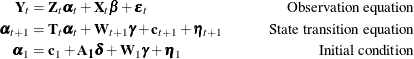
The following list describes these equations:
-
The observation equation describes the relationship between the
 -dimensional response vector
  and the unobserved vectors
  ,
,  , and
, and  . The q-variate responses are vertically stacked in a column to form this -dimensional response vector . The m-dimensional vectors are called states, the k-dimensional vector is the regression coefficient vector associated with predictors
  , and the -dimensional vectors
  are called the observation disturbances. The matrices
  (of dimension
  ) and
) and  (of dimension
  ) correspond to the state effect and the regression effect, respectively. The elements of are assumed to be fully known. The states and the disturbances are random sequences. It is assumed that is a sequence of independent, zero-mean, Gaussian random vectors with diagonal covariances, with the diagonal elements denoted
by
) correspond to the state effect and the regression effect, respectively. The elements of are assumed to be fully known. The states and the disturbances are random sequences. It is assumed that is a sequence of independent, zero-mean, Gaussian random vectors with diagonal covariances, with the diagonal elements denoted
by  .
.
-
The state sequence
is assumed to follow a Markovian structure described by the state transition equation and the associated initial condition.
-
The state transition equation postulates that a new instance of the state,
 , is obtained by multiplying its previous instance,
  , by an m-dimensional square matrix
  (called the state transition matrix) and by adding three more terms: a known nonrandom vector
  (called the state input); a regression term
  , where
  is an
is an  -dimensional design matrix with fully known elements and
  is the g-dimensional regression vector; and a random disturbance vector
  . The m-dimensional state disturbance vectors
  are assumed to be independent, zero-mean, Gaussian random vectors with covariances
  (not necessarily diagonal).
-
The initial condition describes the starting condition of the state evolution equation. The starting state vector
 is assumed to be partially diffuse: it is the sum of a known nonrandom vector
  , a mean-zero Gaussian vector
  , and the terms
  and
and  . represents the contribution from a d-dimensional diffuse vector
  (a diffuse vector is a Gaussian vector with infinite covariance). The observation and state regression vectors
  and
and  are also assumed to be diffuse. The
  matrix
  is assumed to be completely known.
-
The observation disturbances
and the state disturbances (for  ) are assumed to be mutually independent. Either the elements of the matrices
  , , and and the diagonal elements of the observation disturbance covariances
  are assumed to be completely known, or some of them can be functions of a small set of unknown parameters (to be estimated
from the data). Suppose that this unknown set of parameters is denoted by
are assumed to be completely known, or some of them can be functions of a small set of unknown parameters (to be estimated
from the data). Suppose that this unknown set of parameters is denoted by  .
.
-
The d-dimensional diffuse vector
from the state initial condition together with the observation and state regression vectors and constitute the overall  -dimensional diffuse initial condition of the model. See the section Filtering, Smoothing, Likelihood, and Structural Break Detection for more information.
Although this description of the state space model might appear involved, it conveniently covers many variants of the SSMs
that are encountered in practice and precisely describes the most general case that can be handled by the SSM procedure. An
important restriction about the preceding description of the model formulation is that it assumes that the matrices ![]() and
and ![]() that appear in the observation equation and the state equation respectively are free of unknown parameters and that the covariances
of the observation disturbances
that appear in the observation equation and the state equation respectively are free of unknown parameters and that the covariances
of the observation disturbances ![]() are diagonal. In most practical situations, the model under consideration can be easily reformulated to a statistically equivalent
form that conforms to this restriction.
are diagonal. In most practical situations, the model under consideration can be easily reformulated to a statistically equivalent
form that conforms to this restriction.
Note: The transition matrix ![]() in the state equation relates the state
in the state equation relates the state ![]() at time t with the state
at time t with the state ![]() at time
at time ![]() . In many situations, such as when the observations are taken at irregular time intervals,
. In many situations, such as when the observations are taken at irregular time intervals, ![]() depends on information at both t and
depends on information at both t and ![]() . Therefore, it is more appropriate to denote the transition matrix as
. Therefore, it is more appropriate to denote the transition matrix as ![]() . However, for simplicity, the former notation is used throughout this chapter. The same comment applies to the covariance
matrix
. However, for simplicity, the former notation is used throughout this chapter. The same comment applies to the covariance
matrix ![]() of the disturbance term
of the disturbance term ![]() .
.
For easy reference, Table 27.4 summarizes the information contained in the SSM equations.
Table 27.4: State Space Model: Notation
|
Notation |
Description |
|---|---|
|
|
Distinct index values at which the observations are recorded |
|
n |
Number of distinct index instances |
|
|
Number of observations recorded at index |
|
q |
Number of response variables in the model |
|
|
Vertically stacked vector of response values recorded at |
|
|
Total number of response values in the data set |
|
k |
Number of predictor (regressor) variables in the observation equation |
|
|
|
|
|
k-dimensional regression vector that is associated with the predictors |
|
|
|
|
m |
Dimension of the state vectors |
|
|
m-dimensional state vector |
|
|
|
|
|
|
|
|
m-dimensional state input vector |
|
|
|
|
|
g-dimensional state regression vector |
|
|
m-dimensional state disturbance vector |
|
d |
Dimension of the diffuse vector |
|
|
Diffuse vector in the state initial condition |
|
|
|
|
|
m-dimensional state disturbance vector in the initial condition |
|
|
Parameter vector |