The SSM Procedure
-
Overview

- Getting Started
-
Syntax
-
DetailsState Space Model and NotationTypes of Sequence DataOverview of Model Specification SyntaxFiltering, Smoothing, Likelihood, and Structural Break DetectionEstimation of User-Specified Linear Combination of State ElementsContrasting PROC SSM with Other SAS Procedures Predefined Trend ModelsPredefined Structural ModelsCovariance ParameterizationMissing ValuesComputational IssuesDisplayed OutputODS Table NamesODS Graph NamesOUT= Data Set
-
ExamplesBivariate Basic Structural Model Panel Data: Random-Effects and Autoregressive ModelsBackcasting, Forecasting, and InterpolationLongitudinal Data: Smoothing of Repeated MeasuresA User-Defined Trend ModelModel with Multiple ARIMA ComponentsDynamic Factor ModelingDiagnostic Plots and Structural Break AnalysisLongitudinal Data: Variable Bandwidth SmoothingA Transfer Function Model for the Gas Furnace DataPanel Data: Dynamic Panel Model for the Cigar DataMultivariate Modeling: Long-Term Temperature TrendsBivariate Model: Sales of Mink and Muskrat FursFactor Model: Now-Casting the US EconomyLongitudinal Data: Lung Function Analysis
- References
This example shows how you can fit the dynamic Nelson-Siegel (DNS) factor model discussed in Koopman, Mallee, and van der
Wel (2010). The following DATA step creates the yield-curve data set, Dns, that is used in this article. The data are monthly bond yields that were recorded between the start of 1970 to the end of
2000 for 17 bonds of different maturities; the maturities range from three months to 10 years (120 months). The variable date contains the observation date, yield contains the bond yield, maturity contains the associated bond maturity, and mtype contains an index (ranging from 1 to 17) that sequentially labels bonds of increasing maturity. The data have been extended
for two more years by adding missing yields for the years 2001 and 2002, which causes the SSM procedure to produce model forecasts
for this span.
data Dns;
input date : date. yield maturity mtype;
format date date.;
datalines;
1-Jan-70    8.019    3    1
1-Jan-70    8.091    6    2
1-Jan-70    8.108    9    3

   ... more lines ...
In addition, suppose you are interested in extrapolating the fitted model to predict the yield of a hypothetical bond that
has a maturity of 42 months and is not traded on the general exchange. The following DATA step creates the necessary missing
values for this new bond, which is assigned the index of 18—that is, the value of mtype is 18.
data tmp1;
   set dns(keep=date);
   by date;
   if first.date then do;
       yield = .;
       maturity = 42;
       mtype = 18;
       output;
   end;
run;
 proc append data=tmp1 base=dns; run;
 proc sort data=dns;
 by date;
 run;
Suppose that ![]() denotes the (idealized) yield at time t that is associated with a bond of maturity
denotes the (idealized) yield at time t that is associated with a bond of maturity ![]() (in months). Even if time is not measured continuously and the bonds of only certain maturities are traded,
(in months). Even if time is not measured continuously and the bonds of only certain maturities are traded, ![]() is treated as a smooth function of two continuous variables, time t and maturity
is treated as a smooth function of two continuous variables, time t and maturity ![]() . Koopman, Mallee, and van der Wel (2010) discuss a variety of models for
. Koopman, Mallee, and van der Wel (2010) discuss a variety of models for ![]() , which is called the yield surface. One of these models depends on a positive, time-varying, scalar parameter
, which is called the yield surface. One of these models depends on a positive, time-varying, scalar parameter ![]() and a time-varying three-dimensional vector parameter
and a time-varying three-dimensional vector parameter ![]() . This model can be described as follows:
. This model can be described as follows:
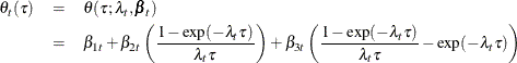
This model is a dynamic version of a static model discussed in Nelson and Siegel (1987), where ![]() and
and ![]() are time invariant. For fixed time period t, the three terms in this model have relatively simple interpretation. The first term
are time invariant. For fixed time period t, the three terms in this model have relatively simple interpretation. The first term ![]() can be thought of as the overall yield level because it does not depend on
can be thought of as the overall yield level because it does not depend on ![]() , the bond maturity. It can also be thought of as the long term yield because as
, the bond maturity. It can also be thought of as the long term yield because as ![]() the other two terms vanish; the coefficients of both
the other two terms vanish; the coefficients of both ![]() and
and ![]() converge to 0 as
converge to 0 as ![]() (recall that
(recall that ![]() is positive). Next, note that as
is positive). Next, note that as ![]() the coefficient of
the coefficient of ![]() in the second term converges to 1 while that of
in the second term converges to 1 while that of ![]() in the third term converges to 0; therefore the second term can be thought of as a correction to the overall yield that is
associated with the short term bonds. Finally, note that the coefficient of
in the third term converges to 0; therefore the second term can be thought of as a correction to the overall yield that is
associated with the short term bonds. Finally, note that the coefficient of ![]() in the third term is a unimodal function of
in the third term is a unimodal function of ![]() that decays monotonically to 0 as
that decays monotonically to 0 as ![]() and as
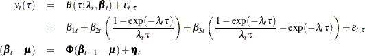
and as ![]() ; therefore the third term is associated with the medium term bond yields. It is postulated that the observed yield, denoted
by
; therefore the third term is associated with the medium term bond yields. It is postulated that the observed yield, denoted
by ![]() , is a noisy version of this unobserved (true) yield
, is a noisy version of this unobserved (true) yield ![]() . The observed yield can be modeled as
. The observed yield can be modeled as
where ![]() are zero-mean, independent, Gaussian variables with variance
are zero-mean, independent, Gaussian variables with variance ![]() , and
, and ![]() is a three-dimensional, Gaussian white noise. That is,
is a three-dimensional, Gaussian white noise. That is, ![]() is a VAR(1) process with mean vector
is a VAR(1) process with mean vector ![]() . The remainder of this example explains how to use the SSM procedure to fit this model to the yield data in the
. The remainder of this example explains how to use the SSM procedure to fit this model to the yield data in the Dns data set.
Suppose that variables Z1, Z2, and Z3 are defined as the coefficients of ![]() ,
, ![]() , and
, and ![]() , respectively. That is,
, respectively. That is,
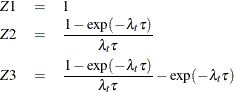
In this case,
Let ![]() . Then
. Then ![]() is a zero-mean VAR(1) process and
is a zero-mean VAR(1) process and ![]() . In particular,
. In particular,
This shows that the model for ![]() can be cast into a state space form with the following observation equation:
can be cast into a state space form with the following observation equation:
The underlying six-dimensional state vector ![]() is formed by joining the two independent subvectors,
is formed by joining the two independent subvectors, ![]() (which is a zero-mean, VAR(1) process) and the constant mean vector
(which is a zero-mean, VAR(1) process) and the constant mean vector ![]() . That is,
. That is, ![]() .
.
Note that the variables Z2 and Z3 depend on the time varying parameter ![]() , which is unknown.
, which is unknown. ![]() is assumed to be a smooth and positive function of time t. In what follows
is assumed to be a smooth and positive function of time t. In what follows ![]() is represented as an exponential of a cubic spline—a B-spline— in time with four evenly spaced interior knots between January
1970 and December 2002. A cubic spline with four interior knots can be represented as a sum of seven (number of knots + spline
degree + 1) B-spline basis functions,
is represented as an exponential of a cubic spline—a B-spline— in time with four evenly spaced interior knots between January
1970 and December 2002. A cubic spline with four interior knots can be represented as a sum of seven (number of knots + spline
degree + 1) B-spline basis functions, ![]() , for example. More specifically,
, for example. More specifically, ![]() can be expressed as
can be expressed as
for some parameters ![]() and the B-spline basis functions (of time)
and the B-spline basis functions (of time) ![]() . Thus, the variables
. Thus, the variables Z2 and Z3 become known functions of time, except for the parameters ![]() , which are estimated from the data. The following statements augment the
, which are estimated from the data. The following statements augment the Dns data set with the B-spline basis columns in two steps. First a data set that contains the basis columns, c1–c7, is created by using the BSPLINE function in the IML procedure. This data set is then merged with the Dns data set.
 proc iml;
    use dns;
    read all var {date} into x;
    bsp = bspline(x, 2, ., 4);
    create spline var{c1 c2 c3 c4 c5 c6 c7};
    append from bsp;
 quit;
 data dns;
    merge dns spline;
 run;
The following statements use the SSM procedure to perform the model fitting and forecasting calculations. The variance of
the observation equation disturbance for the hypothetical bond (mtype = 18) is taken to be the average of the neighboring bonds (mtype = 10 and 11), whose maturities are 36 and 48 months, respectively.
  proc ssm data=Dns optimizer(technique=dbldog maxiter=400);
       id date interval=month;

      /* Time-varying parameter lambda */
      parms v1-v7;
      lambda = exp(v1*c1 + v2*c2 + v3*c3 + v4*c4
           + v5*c5 + v6*c6 + v7*c7);

      /* Observation equation disturbance -- separate variance for each maturity */
      parms sigma1-sigma17 / lower=1.e-4;
      array s_array(17) sigma1-sigma17;
       do i=1 to 17;
          if (mtype=i) then sigma = s_array[i];
       end;
       if (mtype=18) then sigma = (sigma10+sigma11)/2;
       irregular wn variance=sigma;

       /* Variables Z1, Z2, Z3 needed in the observation equation */
       Z1= 1.0;
       tmp = lambda*maturity;
       Z2 = (1-exp(-tmp))/tmp;
       Z3 = ( 1-exp(-tmp)-tmp*exp(-tmp) )/tmp;

        /* Zero-mean VAR(1) factor zeta and the associated component */
       state zeta(3) type=VARMA(p(d)=1) cov(g) print=(cov ar);
       comp zetaComp = (Z1-Z3)*zeta;

       /* Constant mean vector mu and the associated component */
        state mu(3) type=rw;
        comp muComp = (Z1-Z3)*mu;

        /* Observation equation */
        model yield = muComp zetaComp wn;

        /* Various components defined only for output purposes  */
        eval yieldSurface = muComp + zetaComp;

        comp zeta1 = zeta[1];
        comp zeta2 = zeta[2];
        comp zeta3 = zeta[3];
        comp mu1 = mu[1];
        comp mu2 = mu[2];
        comp mu3 = mu[3];

        comp z2zeta = (Z2)*zeta[2];
        comp z3zeta = (Z3)*zeta[3];
        comp z2Mu =  (Z2)*mu[2];
        comp z3Mu =  (Z3)*mu[3];

        eval beta1 = mu1 + zeta1;
        eval beta2 = mu2 + zeta2;
        eval beta3 = mu3 + zeta3;

        eval shortTem = z2zeta + z2Mu;
        eval medTerm = z3zeta + z3Mu;

        /* output the component estimates and the forecasts */
        output out=dnsFor pdv;
    run;
The DBLDOG optimization technique is used for parameter estimation since it is computationally more efficient in this example.
The transition matrix, ![]() , in the VAR(1) specification of
, in the VAR(1) specification of ![]() is taken to be diagonal (TYPE=VARMA(P(D)=1)) because the use of more general square matrix did not improve the model fit
significantly. The mean vector
is taken to be diagonal (TYPE=VARMA(P(D)=1)) because the use of more general square matrix did not improve the model fit
significantly. The mean vector ![]() (recall that
(recall that ![]() ) is specified as a three-dimensional random walk with zero disturbance covariance (signified by the absence of COV= option).
The model specification part of the program ends with the MODEL statement; the subsequent COMP and EVAL statements define
some useful linear combinations of the underlying state. Their estimates are computed after the model fit is completed and
are output to the output data set
) is specified as a three-dimensional random walk with zero disturbance covariance (signified by the absence of COV= option).
The model specification part of the program ends with the MODEL statement; the subsequent COMP and EVAL statements define
some useful linear combinations of the underlying state. Their estimates are computed after the model fit is completed and
are output to the output data set dnsFor. The dnsFor data set also contains all the program variables and the parameters defined in the PARMS statement because the OUTPUT statement
contains the PDV option.
Output 27.7.1 shows the estimated mean vector (![]() ). It shows that the mean long-term yield is 7.64. Output 27.7.2 shows the estimates of
). It shows that the mean long-term yield is 7.64. Output 27.7.2 shows the estimates of v1–v7 (used for defining time-varying ![]() ) and the maturity specific observation variances. Output 27.7.3 shows the estimate of the VAR(1) transition matrix
) and the maturity specific observation variances. Output 27.7.3 shows the estimate of the VAR(1) transition matrix ![]() , and Output 27.7.4 shows the associated disturbance covariance matrix
, and Output 27.7.4 shows the associated disturbance covariance matrix ![]() . The model fit summary is shown in Output 27.7.5.
. The model fit summary is shown in Output 27.7.5.
Output 27.7.2: Estimates of v1–v7 and Observation Variances
| Estimates of Named Parameters | ||
|---|---|---|
| Parameter | Estimate | Standard Error |
| v1 | -1.19587 | 0.304003 |
| v2 | -2.93679 | 0.111440 |
| v3 | -1.88709 | 0.068972 |
| v4 | -2.31371 | 0.079116 |
| v5 | -3.21875 | 0.105575 |
| v6 | -1.66055 | 0.315692 |
| v7 | -4.60122 | 1.548096 |
| sigma1 | 0.05406 | 0.004708 |
| sigma2 | 0.00349 | 0.000865 |
| sigma3 | 0.00869 | 0.000752 |
| sigma4 | 0.01093 | 0.000901 |
| sigma5 | 0.00865 | 0.000757 |
| sigma6 | 0.00603 | 0.000571 |
| sigma7 | 0.00519 | 0.000491 |
| sigma8 | 0.00542 | 0.000497 |
| sigma9 | 0.00562 | 0.000500 |
| sigma10 | 0.00639 | 0.000559 |
| sigma11 | 0.01032 | 0.000848 |
| sigma12 | 0.00742 | 0.000676 |
| sigma13 | 0.01106 | 0.000947 |
| sigma14 | 0.01194 | 0.001051 |
| sigma15 | 0.01244 | 0.001162 |
| sigma16 | 0.02140 | 0.001842 |
| sigma17 | 0.02746 | 0.002295 |
The following statements produce the time series plots of the smoothed estimate of the idealized bond yield (![]() ) for bonds with maturities 30, 60, and 120 months (shown in Output 27.7.6). To simplify the display, the plots exclude the time span prior to 1991.
) for bonds with maturities 30, 60, and 120 months (shown in Output 27.7.6). To simplify the display, the plots exclude the time span prior to 1991.
 proc sgplot data= dnsFor;
     title "The Estimated Yield Surface and the Observed Yields ";
     where maturity in (3 60 120) and date >= '31dec1990'd;
     series x=date y=smoothed_yieldSurface / group=maturity;
     scatter x=date y=yield / group=maturity;
     refline '31dec2000'd / axis=x lineattrs=GraphReference(pattern = Dash)
         name="RefLine"   label="Start of multistep forecasts";
 run;
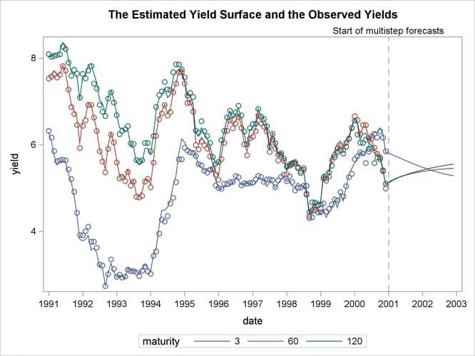
The plots indicate that the DNS model is a reasonable description of the yield data. Similar plots (not shown here) for other
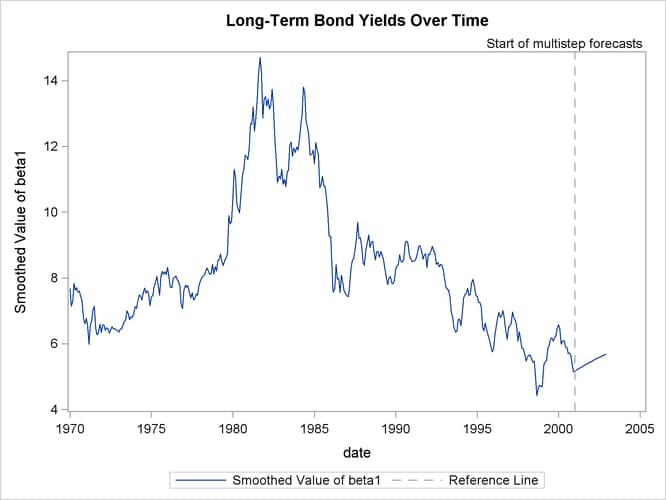
maturities also indicate the adequacy of the DNS model. The following statements produce the time series plot of the smoothed
estimate of ![]() , the long-term bond yield (shown in Output 27.7.7) :
, the long-term bond yield (shown in Output 27.7.7) :
 proc sgplot data=dnsFor;
    title "Long-Term Bond Yields Over Time ";
    series x=date y=smoothed_beta1 ;
    refline '31dec2000'd / axis=x lineattrs=GraphReference(pattern = Dash)
         name="RefLine"   label="Start of multistep forecasts";
 run;
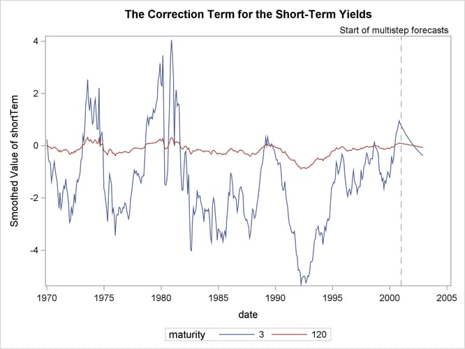
Similarly, Output 27.7.8, which is produced by the following statements, shows the smoothed estimate of the correction to the overall yield that is
provided by the second term (![]() ) for maturities of 3 months and 120 months. As expected, the correction for the (long-term) maturity of 120 months is negligible
compared to the (short-term) maturity of 3 months.
) for maturities of 3 months and 120 months. As expected, the correction for the (long-term) maturity of 120 months is negligible
compared to the (short-term) maturity of 3 months.
 proc sgplot data=dnsFor;
   title "The Correction Term for the Short-Term Yields ";
   where maturity in (3 120);
   series x=date y=smoothed_shortTem / group=maturity;
   refline '31dec2000'd / axis=x lineattrs=GraphReference(pattern = Dash)
         name="RefLine"   label="Start of multistep forecasts";
 run;
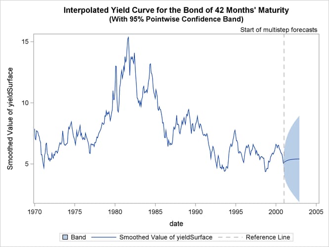
The following statements create plots that show the estimated yield for the hypothetical bond whose maturity is 42 months:
proc sgplot data=dnsFor;
   title "Interpolated Yield Curve for the Bond of 42 Months' Maturity";
   title2 "(With 95% Pointwise Confidence Band)";
   where maturity in (42);
   band x=date lower=smoothed_lower_yieldSurface upper=smoothed_upper_yieldSurface;
   series x=date y=smoothed_yieldSurface;
   refline '31dec2000'd / axis=x lineattrs=GraphReference(pattern = Dash)
      name="RefLine"   label="Start of multistep forecasts";
run;
proc sgplot data= dnsFor;
  title "Estimated Yield Curves";
  title2 "(Maturities 36, 42, and 48 Months)";
  where maturity in (36 42 48) and date >= '31dec1990'd;
  series x=date y=smoothed_yieldSurface / group=maturity;
  refline '31dec2000'd / axis=x lineattrs=GraphReference(pattern = Dash)
      name="RefLine"   label="Start of multistep forecasts";
run;
Output 27.7.9 shows the interpolated yield curve with a pointwise 95% confidence band. In the historical period, the confidence band appears too tight, mostly because of graphical scaling.
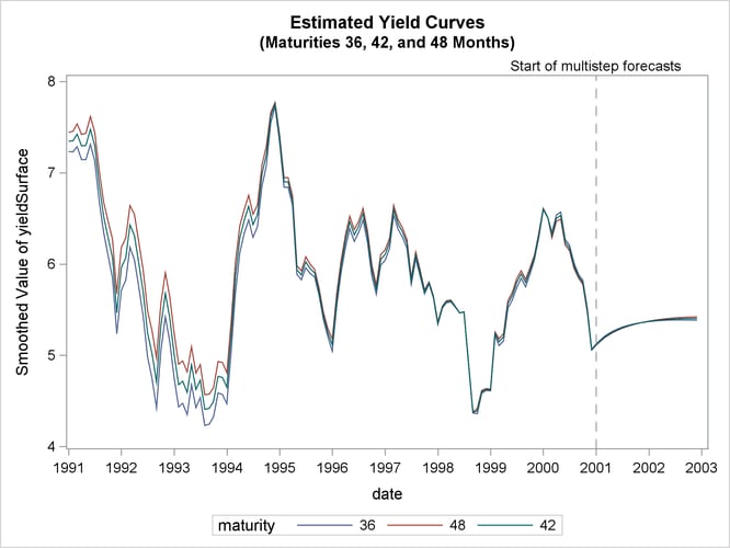
Output 27.7.10 shows the estimates of ![]() for
for ![]() = 36, 42, and 48 months. As expected, the estimated
= 36, 42, and 48 months. As expected, the estimated ![]() lies between the estimates of
lies between the estimates of ![]() and
and ![]() .
.