The SSM Procedure

This example illustrates how you can use the SSM procedure to analyze a panel of time series. The following data set, Cigar, contains information about yearly per capita cigarette sales for 46 geographic regions in the United States over the period 1963–1992. The variables lsales, lprice, lndi, and lpimin denote the per capita cigarette sales, price per pack of cigarettes, per capita disposable income, and minimum price in adjoining regions per pack of cigarettes, respectively (all in the natural log scale). The variable year contains the observation year, and the variable region contains an integer between 1 to 46 that serves as the unique identifier for the region. For additional data description see Baltagi and Levin (1992); Baltagi (1995). The data are sorted by year.

data cigar;
    input year region lsales lprice lndi lpimin;
    label lsales = 'Log cigarette sales in packs per capita';
    label lprice = 'Log price per pack of cigarettes';
    label lndi = 'Log per capita disposable income';
    label lpimin = 'Log minimum price in adjoining regions
                     per pack of cigarettes';
    year = intnx( 'year', '1jan63'd, year-63 );
    format year year.;
datalines;
63 1 4.54223 3.35341 7.3514 3.26194
63 2 4.82831 3.17388 7.5729 3.21487
63 3 4.63860 3.29584 7.3000 3.25037
63 4 4.95583 3.23080 7.9288 3.17388
63 5 5.05114 3.28840 7.9772 3.26576

   ... more lines ...   

The goal of the analysis is to study the impact of the regressors on the smoking behavior and to understand the changes in the smoking patterns in different regions over the years. Consider the following model for lsales:

This model represents lsales in a region i and in a year t as a sum of region-specific trend components , the regression effects due to lprice, lndi, and lpimin, and the observation noise . Different variations of this model are obtained by considering different models for the trend component . Proper modeling of the trend component is important because it captures differences between the regions because of unrecorded factors such as demographic changes over time, results of anti-smoking campaigns, and so on. The following statements specify and fit one such model:

 proc ssm data=Cigar plots=residual;
    id year interval=year;
    array RegionArray{46} region1-region46;
    do i=1 to 46;
       RegionArray[i] = (region=i);
    end;
    trend IrwTrend(ll) cross(matchparm)=(RegionArray) levelvar=0;
    irregular wn;
    model lsales = lprice lndi lpimin IrwTrend wn;
    eval TrendPlusReg = IrwTrend + lprice + lndi + lpimin;
    output out=forCigar pdv press;
 run;

The PROC SSM statement specifies the input data set, Cigar, which contains analysis variables such as the response variable, lsales, and the predictor variables, lprice, lndi, and lpimin. The PLOTS=RESIDUAL option in the PROC SSM statement produces residual diagnostic plots. The optional ID statement specifies a numeric index variable (often a SAS date or datetime variable), which is year in this case. The INTERVAL=YEAR option in the ID statement indicates that the measurements are collected on a yearly basis. The next few statements define a 46-dimensional array of dummy variables, RegionArray, such that RegionArray[i] is 1 if region is i and is 0 otherwise. The next three statements, TREND, IRREGULAR, and MODEL, constitute the model specification part of the program:

The last two statements, EVAL and OUTPUT, control certain aspects of the procedure output. The following EVAL statement defines a linear combination, named TrendPlusReg, of selected terms in the MODEL statement.

     eval TrendPlusReg = IrwTrend + lprice + lndi + lpimin;

This EVAL statement causes the SSM procedure to produce an estimate of TrendPlusReg (and its standard error), which can then be printed or output to a data set. TrendPlusReg contains all the terms in the model except for the observation noise and thus can be regarded as the explanatory part of the model. In the OUTPUT statement, you can specify an output data set that stores all the component estimates that are produced by the procedure. The following OUTPUT statement specifies forCigar as the output data set:

     output out=forCigar pdv press;
  

The PDV option causes variables such as region1–region46, which are defined by the DATA step statements within the SSM procedure, also to be included in the output data set. The PRESS option causes the printing of fit measures that are based on the delete-one cross validation errors (see the section Delete-One Cross Validation and Structural Breaks for more information).

All the models that are specified in the SSM procedure possess a state space representation. See the section State Space Model and Notation for more information. The SSM procedure output begins with a table (not shown here) of the input data set that provides the name and other information. Next, the "Model Summary" table, shown in Figure 27.1, provides basic model information, such as the following:

This information is very useful in determining the computational complexity of the model (the larger state size, 92, explains the relatively long computing time—as much as two minutes on some desktops—for this example).

The index variable information is shown in Figure 27.2. Among other things, it categorizes the data to be of the type Regular with Replication, which implies that the data are regularly spaced with respect to the ID variable and at least some observations have the same ID value. This is clearly true in this example: the data are yearly without any gaps, and there are 46 observations in each year—one per region.

Figure 27.3 provides simple summary information about the response variable. It shows that lsales has no missing values and no induced missing values because the predictors in the model, lprice, lndi, and lpimin, do not have any missing values either.

The regression coefficients of lprice, lndi, and lpimin are shown in Figure 27.4. As expected, the coefficient of lprice is negative and the coefficients of lndi and lpimin are positive, all being statistically significant. This is consistent with the expectation that the cigarette sales are adversely affected by the price and are positively correlated with the disposable income. The estimated effect of lpimin, called bootlegging effect by Baltagi and Levin (1992), is statistically significant but much smaller than the effects of lprice and lndi.

Figure 27.5 shows the estimates of the disturbance variance of the slope equation in IrwTrend and the variance of the noise term wn. The estimate of the disturbance variance of the slope equation in IrwTrend, 0.00017, is statistically significant (being several times larger than its standard error, 0.000022). This implies that the estimated trends are not simple lines with fixed intercept and slope.

Figure 27.6 shows a panel of residual normality diagnostic plots. These plots show that the residuals are symmetrically distributed but contain slightly larger than expected number of extreme residuals. Figure 27.7 shows the plot of residuals versus time. There the residuals do not exhibit any obvious pattern; however, the plot does show that more extreme residuals appear before 1970 and after 1989. On the whole, however, these plots do not exhibit serious violations of model assumptions.

Figure 27.6: Residual Normality Check

Figure 27.7: Standardized Residuals Plotted against Time

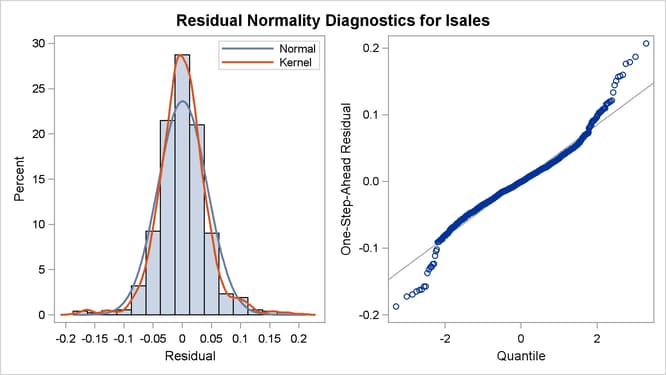
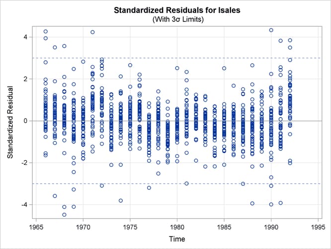
Figure 27.8 shows the details of the likelihood computations such as the number of nonmissing response values used and the likelihood of the fitted model. See the section Likelihood Computation and Model Fitting Phase for more information. Figure 27.8 shows the likelihood-based information criteria in lower-is-better format, which are useful for model comparison.

In addition to the regression estimates, it is useful to analyze the estimates of different model components such as the trend component IrwTrend and the linear combination TrendPlusReg. These estimates can be printed by using the PRINT= option provided in the TREND and EVAL statements, or they can be output to a data set (as it is done in this illustration). This latter option is particularly useful for graphical exploration of these components by standard graphical procedures such as SGPLOT and SGPANEL procedures. The following statements produce a panel of plots that shows how well the proposed model fits the observed cigarette sales in the first three regions, which correspond to Alabama, Arizona, and Arkansas. The output data set, forCigar, contains all the needed information: Smoothed_TrendPlusReg contains the smoothed (full-sample) estimate of TrendPlusReg, and Smoothed_Lower_TrendPlusReg and Smoothed_Upper_TrendPlusReg contain its 95% lower and upper confidence limits. In addition, for easy readability, a user-defined format (RegionFormat), which is created by using the FORMAT procedure (not shown), is used to associate the region names to region values.

proc sgpanel data=forCigar noautolegend;
   where region <= 3;
   format region RegionFormat.;
   title 'Region-Specific Sales Patterns with 95% Confidence Band';
   panelby region / columns=3;
   band x=year lower=Smoothed_Lower_TrendPlusReg
   upper=Smoothed_Upper_TrendPlusReg;
   scatter x=year y=lsales;
   series x=year y= Smoothed_TrendPlusReg;
run;

Figure 27.10: Cigarette Sales Patterns for the First Three Regions

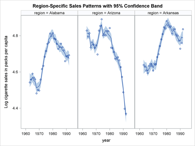
Figure 27.10 seems to indicate that the model fits the data reasonably well. It also shows that Arizona differs markedly from Alabama and Arkansas in its cigarette sales pattern over the years. The following statements produce a similar panel of plots that show the estimate of trend without the regression effects:

proc sgpanel data=forCigar noautolegend;
   where region <= 3;
   format region RegionFormat.;
   title 'Region-Specific Trend Estimates';
   panelby region / columns=3;
   series x=year y= smoothed_IrwTrend;
run;

Figure 27.11: Estimate of IrwTrend for the First Three Regions

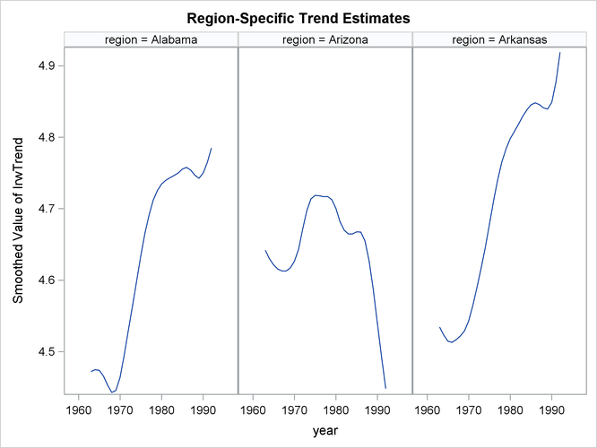
The trend patterns, shown in Figure 27.11, seem to suggest that after accounting for the regression effects, per capita cigarette sales were on the rise in Alabama and Arkansas while they were declining in Arizona.