The SSM Procedure

Example 27.12 Multivariate Modeling: Long-Term Temperature Trends

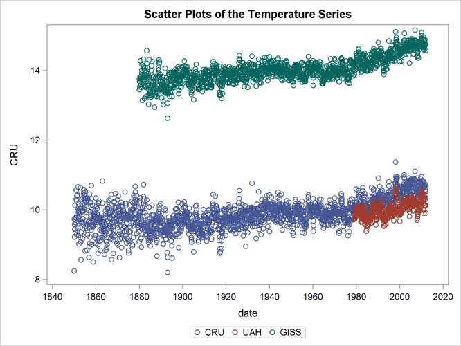
In a presentation by Ansley and de Jong (2012), three monthly time series are jointly modeled to obtain long-term—several decades long—temperature predictions for certain regions of the northern hemisphere. This example shows how you can specify and fit the final model that this presentation proposed. The following data set, Temp, contains four variables: date dates the monthly observations; UAH contains monthly satellite global temperature readings, starting in December 1978; CRU contains monthly temperature data, starting in January 1850 (from a different source); and GISS contains monthly temperature data, starting in January 1880 (from yet another source). All these temperature data are scaled suitably so that the numbers represent temperature readings in centigrade.

data Temp;
input UAH CRU GISS @@;
date = intnx('month', '01jan1850'd, _n_-1);
format date date.;
datalines;
.    8.243    .
.    9.733    .

   ... more lines ...

The following statements produce scatter plots of these three series in a single graph:

 proc sgplot data=Temp;
       title "Scatter Plots of the Temperature Series";
       scatter x=date y=cru;
       scatter x=date y=uah ;
       scatter x=date y=giss;
  run;

Output 27.12.1 shows the resulting graph. As already noted, these three series start at different points in the past. However, they all end at the same time: they all have measurements until January 2012, which is the last month in the data set. The mean levels of these series are different: the GISS measurements are generally larger than CRU and UAH by about 4 degrees. In addition, the variability in the CRU values seems to decrease with time (this is more apparent when the series is plotted by itself). The goal of the analysis is to use these data to make long-term predictions about future temperature levels. The following statements append 1,200 missing measurements to Temp, so that the model fitted by using the SSM procedure can be extrapolated to obtain temperature forecasts 100 years in the future:

data append(keep=date cru giss uah);
    do i=1 to 1200;
        cru = .; giss=.; uah=.;
        date = intnx('month','01jan2012'D, i);
    format date monyy7.;
    output;
    end;
run;

 proc append base=Temp data=Append; run;

Output 27.12.1: Scatter Plots of CRU, UAH, and GISS

Ansley and de Jong propose a parsimonious model that links these three time series. It can be described as

$\begin{eqnarray*} \mr{GISS}_{t} & = & \mu _{t} + a \; \zeta _{t} + a\; r_{1}\; \epsilon _{1 t} \nonumber \\ \mr{CRU}_{t} & = & \beta _{cru} + \mu _{t} + a \; \zeta _{t} + a\; \epsilon _{2 t} \nonumber \\ \mr{UAH}_{t} & = & \beta _{uah} + \mu _{t} + a \; \zeta _{t} + a\; r_{3}\; \epsilon _{3 t} \nonumber \end{eqnarray*}$

where $\beta _{cru}$ and $\beta _{uah}$ are intercepts that are associated with CRU and UAH, respectively; $\mu _{t}$ is an integrated random walk trend; $\zeta _{t}$ is a zero-mean, autoregressive noise term (which is scaled by an unknown scaling factor a); and $\epsilon _{i t}$ ( $i = 1, 2, 3$ ) are independent observation errors with different variances that are also scaled suitably. Note that the trend $\mu _{t}$ and the autoregressive noise term $\zeta _{t}$ are shared by the models of the three series, and, for identification purposes, the intercept for GISS is taken to be zero. In addition, the model parameters are assumed to be interrelated and are parameterized in a particular way (which leads to fewer parameters to estimate, and their relative scaling helps in parameter estimation). This special parameterization can be expressed as a function of seven basic parameters: loga1, logr1, logr3, logsigma, b, c, and rhoParm (this naming convention is different from that used by Ansley and de Jong (2012)).

Let $\sigma ^{2} = \exp (2 \text {logsigma})$ , and let the scaling factors $a = \exp (\text {loga1})$ , $r_{1} = \exp (\text {logr1})$ , and $r_{3} = \exp ( \text {logr3})$ . Then the model parameters can be described as follows:

The parameters that are associated with the autoregression $\zeta _{t}$ : the damping factor 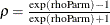$\rho = \frac{ \exp (\text {rhoParm})-1}{\exp (\text {rhoParm})+1}$ , the variance of the disturbance term = $a^{2} \sigma ^{2}$ , and the variance of the initial state = $a^{2} \sigma ^{2}/(1 - \rho ^{2})$
The parameters that are associated with the integrated random walk trend: the variance of the disturbance term in the slope equation = $\sigma ^{2}$
The variance of the observation errors for GISS = $a^{2} r_{1}^{2} \sigma ^{2}$
The variance of the observation errors for UAH = $a^{2} r_{3}^{2} \sigma ^{2}$
The variance of the observation errors for CRU is taken to be time-varying with the following form: for $t \leq nobs,$

$\sigma ^{2}_{2, t} = a^{2} \sigma ^{2} \exp (2 b + 2 c\; t / nobs)$

where $nobs$ = 1,945 (the number of observations in the unappended data set). For $t >$ 1,945, it is fixed at its last value: $\sigma ^{2}_{2, t} = a^{2} \sigma ^{2} \exp (2 b + 2 c)$ .

The following DATA step adds an observation index, tindex, to Temp, which is used in the SSM procedure to define the time-varying observation error variance for CRU:

data temp;
   set temp;
   tindex = _n_;
run;

The following statements fit the preceding model to the Temp data:

 ods output RegressionEstimates=regEst;
 proc ssm data=Temp;
     id date interval=month;
     parms loga1 logr1 logr3  logsigma;
     parms b=0 c=0;
     parms rhoParm;
     rho = (exp(rhoParm)-1)/(exp(rhoParm)+1);
     sigmaSq = exp(2*logsigma);
     initSigmaSq = sigmaSq/(1-rho*rho);
     a1 = exp(loga1);
     a1Sq = a1*a1;
     r1sq  = exp(2*logr1);
     r3sq  = exp(2*logr3);
     giss_var = a1Sq*r1sq*sigmaSq;
     nobs=1945;
     if tindex <= nobs then
         cru_var = a1Sq*exp(2*b + 2*c*tindex/nobs)*sigmaSq;
     else cru_var = a1Sq*exp(2*b + 2*c)*sigmaSq;
     uah_var = a1Sq*r3sq*sigmaSq;
     UAH_Intercept=1.0;
     CRU_Intercept=1.0;
     trend level(ll) variance=0 slopevar=sigmaSq;
     state auto(1) T(g)=(rho) cov(g)=(sigmaSq)  cov1(g)=(initSigmaSq);
     comp auto_common = auto*(a1);
     state wn(3) type=wn cov(d)=(giss_var cru_var uah_var);
     comp wn_giss = wn[1];
     comp wn_cru = wn[2];
     comp wn_uah = wn[3];
     model GISS = level auto_common  wn_giss;
     model CRU = CRU_Intercept level auto_common  wn_cru;
     model UAH = UAH_Intercept level auto_common  wn_uah;
     comp slope = level_state_*(0 1);
     output out=For pdv press;
 run;

Output 27.12.2 shows the estimated intercepts $\hat{\beta }_{cru}$ and $\hat{\beta }_{uah}$ . As expected, they are quite close (see the scatter plots of CRU and UAH in Output 27.12.1).

Output 27.12.2: Estimated Intercepts for CRU and UAH

The SSM Procedure

Regression Parameter Estimates
Response Variable	Regression Variable	Estimate	Standard Error	t Value	Pr > \|t\|
CRU	CRU_Intercept	-4.10	0.00360	-1139.2	<.0001
UAH	UAH_Intercept	-4.48	0.00671	-666.48	<.0001

The estimates of the basic parameters that underlie the model parameters are shown in Output 27.12.3.

Output 27.12.3: Estimates of Basic Model Parameters

Estimates of Named Parameters
Parameter	Estimate	Standard Error
loga1	7.820	0.3819
logr1	-1.005	0.0884
logr3	-0.231	0.0453
logsigma	-9.682	0.3806
b	0.737	0.0502
c	-1.403	0.0689
rhoParm	1.432	0.0767

The following DATA steps add two variables (CRU_ADJ = CRU – $\hat{\beta }_{cru}$ and UAH_ADJ = UAH – $\hat{\beta }_{uah}$ ) to the output data set For. These adjusted versions of CRU and UAH have the same mean level as GISS—estimated $\mu _{t}$ .

data _NULL_;
   set regEst;
   if _n_ = 1 then call symput('intercept1',trim(left(estimate)));
   else call symput('intercept2',trim(left(estimate)));
run;
data for;
    set For;
    cru_adj = cru - &intercept1;
    uah_adj = uah - &intercept2;
run;

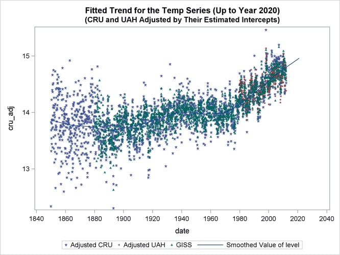
The following statements produce a graph that contains four plots: scatter plots of GISS, CRU_ADJ, and UAH_ADJ and a series plot of the estimated $\mu _{t}$ .

 proc sgplot data=For;
    where date < '01feb2021'd;
    title "Fitted Trend for the Temp Series (Up to Year 2020) ";
    title2 "(CRU and UAH Adjusted by Their Estimated Intercepts) ";
    scatter x=date y=cru_adj / LEGENDLABEL="Adjusted CRU"
        MARKERATTRS=GraphData1(symbol=star size=3);
    scatter x=date y=uah_adj / LEGENDLABEL="Adjusted UAH"
        MARKERATTRS=GraphData2(symbol=plus size=3);
    scatter x=date y=giss /
        MARKERATTRS=GraphData3(symbol=triangle size=3);
    series x=date y=smoothed_level / MARKERATTRS=GraphData4;
 run;

Output 27.12.4 shows the resulting graph. It shows that the estimated mean level $\mu _{t}$ tracks the observed data quite well.

Output 27.12.4: Fitted Trend $\mu _{t}$

The following statements produce the time series plot of the estimated $\mu _{t}$ along with the 95% confidence band:

 proc sgplot data=For;
    title "Temperature Projections for the Next 100 Years";
    band x=date lower=smoothed_lower_level upper=smoothed_upper_level;
    series x=date y=smoothed_level;
    refline '01feb2012'd / axis=x lineattrs=(pattern=shortdash)
       LEGENDLABEL= "Start of Multistep Forecasts"
       name="Forecast Reference Line";
 run;

Output 27.12.5 shows the resulting graph.

Output 27.12.5: Long-Term Forecasts of $\mu _{t}$

The following statements produce a similar graph for the estimated slope of $\mu _{t}$ :

 proc sgplot data=For;
    where date <=  '01feb2031'd;
    title "The Monthly Rate of Temperature Change  (Up to Year 2030)";
    band x=date lower=smoothed_lower_slope upper=smoothed_upper_slope;
    series x=date y=smoothed_slope;
    refline '01feb2012'd / axis=x lineattrs=(pattern=shortdash)
       LEGENDLABEL= "Start of Multistep Forecasts"
       name="Forecast Reference Line";
    refline 0 / axis=y lineattrs=(pattern=dash);
 run;

Output 27.12.6 shows the resulting plot of the estimated slope of $\mu _{t}$ .

Output 27.12.6: Forecasts of the Slope of $\mu _{t}$

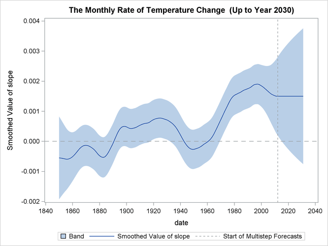
Based on the preceding analysis (see the plots of $\mu _{t}$ and its slope in Output 27.12.5 and Output 27.12.6), it appears that there has been statistically significant warming over the last 10 years, but the warming does not appear to be accelerating.