The SSM Procedure

This example of a repeated measures study is taken from Diggle, Liang, and Zeger (1994, p. 100). The data consist of body weights of 27 cows, measured at 23 unequally spaced time points over a period of approximately 22 months. Following Diggle, Liang, and Zeger (1994), one animal is removed from the analysis, one observation is removed according to their Figure 5.7, and the time is shifted to start at 0 and is measured in 10-day increments. The design is a factorial, and the factors are the infection of an animal with M. paratuberculosis and whether the animal is receiving iron dosing. The data set contains five variables: cow assigns a unique identification number—from 1 to 26—to each cow in the study, tpoint denotes the time of the growth measurement, weight denotes the growth measurement, iron is a dummy variable that indicates whether the animal is receiving iron or not, and infection is a dummy variable that indicates whether the animal is infected or not. The goal of the study is to assess the effect of iron and infection—and their possible interaction—on weight. The following DATA steps create this data set:

data times;
  input time1-time23;
  datalines;
 122  150  166  179  219  247  276  296  324  354  380  445
 478  508  536  569  599  627  655  668  723  751  781
;

data Cows;
  if _n_ = 1 then merge times;
  array t{23} time1   - time23;
  array w{23} weight1 - weight23;
  input cow iron infection weight1-weight23 @@;
  do i=1 to 23;
     weight = w{i};
     tpoint = (t{i}-t{1})/10;
     output;
  end;
  keep cow iron infection tpoint weight;
  datalines;
  1 0 0  4.7    4.905  5.011  5.075  5.136  5.165  5.298  5.323
         5.416  5.438  5.541  5.652  5.687  5.737  5.814  5.799

   ... more lines ...   

The following DATA step adds ironInf, a grouping variable that is used later during the plotting of the results. In the next step, the data are sorted by the index variable, tpoint.

data Cows;
   set Cows;
   ironInf = "No Iron and No Infection";
   if iron=1 and infection=1 then ironInf = "Iron and Infection";
   else if iron=1 and infection=0 then ironInf = "Iron and No Infection";
   else if iron=0 and infection=1 then ironInf = "No Iron and Infection";
   else ironInf = "No Iron and No Infection";
   run;

 proc sort data=Cows;
     by tpoint ;
 run;

To assess the effect of iron and infection on weight, the natural growth profile of the animals must also be accounted for. Here two alternate models for this problem are considered. The first model assumes that the observed weight of an animal is the sum of a common growth profile, which is modeled by a polynomial spline trend of order 2, the regression effects of iron and infection, and the observation error—modeled as white noise. An interaction term, for interaction between iron and infection, was found to be insignificant and is not included. In the second model, the common growth profile and the regression variables of the first model are replaced by four environment specific growth profiles.

The following statements fit the first model:

 proc ssm data=Cows;
    id tpoint;
    trend growth(ps(2));
    irregular wn;
    model weight = iron infection growth wn;
    eval pattern = iron + infection + growth;
    output out=For;
 quit;

Output 27.4.1 shows that the state dimension of this model is 2 (corresponding to the polynomial trend specification of order 2), the number of diffuse elements in the initial condition is 4 (corresponding to the trend and the two regressors iron and infection), and the number of unknown parameters is 2 (corresponding to the variance parameters of trend and irregular).

Output 27.4.2 shows that the ID variable is irregularly spaced with replication.

The estimated regression coefficients of iron and infection, shown in Output 27.4.3, are significant and negative. This implies that both iron and infection adversely affect the response variable, weight.

The variance estimates of the trend component and the irregular component are shown in Output 27.4.4.

After examining the model fit, it is useful to study how well the patterns implied by the model follow the data. pattern, defined by the EVAL statement, is a sum of the trend component and the regression effects. A graphical examination of the smoothed estimate of pattern is done next. The following DATA step merges the output data set specified in the OUTPUT statement, For, with the input data set, Cows. In particular, this adds ironInf (a grouping variable from Cows) to For.

data For;
    merge for Cows;
    by tpoint;
run;

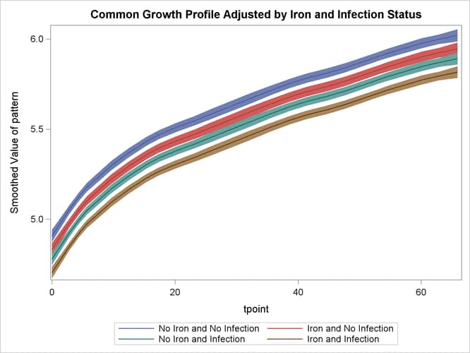
The following statements produce the graphs of smoothed_pattern, grouped according to the environment condition (see Output 27.4.5). The plot clearly shows that the control group "No Iron and No Infection" has the best growth profile, while the worst growth profile is for the group "Iron and Infection."

 proc sgplot data=For noautolegend;
     title 'Common Growth Profile Adjusted by Iron and Infection Status';
     band x=tpoint lower=smoothed_lower_pattern
        upper=smoothed_upper_pattern / group=ironInf name="band";
     series  x=tpoint y=smoothed_pattern / group=ironInf name="series";
     keylegend "series";
 run;

Output 27.4.5: Model 1: Growth Profile Comparison with 95% Confidence Bands

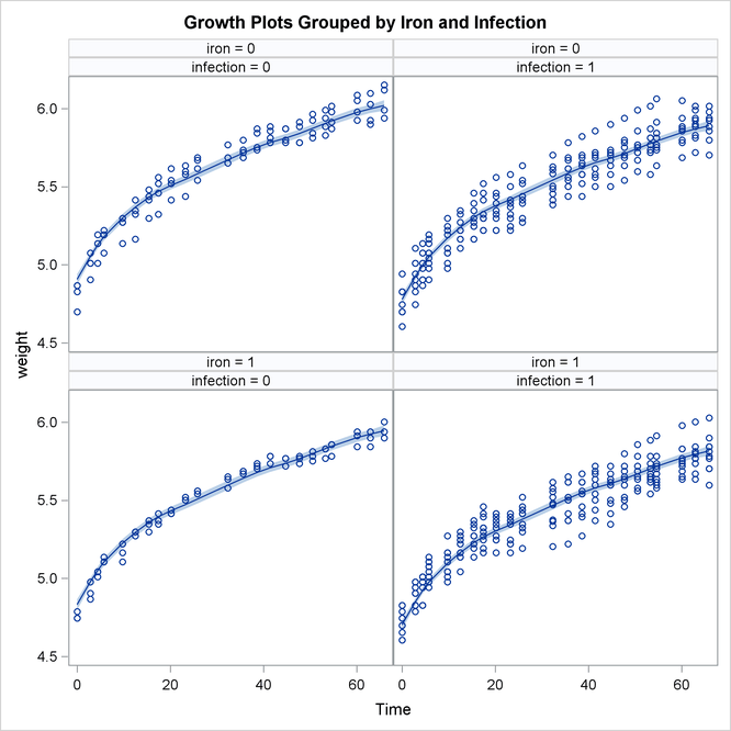
The following statements produce a panel of plots that show how well smoothed_pattern follows the observed data:

 proc sgpanel data=For noautolegend;
   title 'Growth Plots Grouped by Iron and Infection';
    label tpoint='Time' ;
    panelby iron infection / columns=2;
    band x=tpoint lower=smoothed_lower_pattern
       upper=smoothed_upper_pattern ;
    scatter x=tpoint y=weight;
    series  x=tpoint y=smoothed_pattern ;
 run;

Output 27.4.6 shows that the model fits the data reasonably well.

Output 27.4.6: Model 1: Smoothed Model Fit Lines

The following statements fit the second model. In this model separate polynomial trends are fit according to different settings of iron and infection by specifying an appropriate list of (dummy) variables in the CROSS= option of the trend specification.

 proc ssm data=Cows;
     id tpoint;
     a1 = (iron=1 and infection=1);
     a2 = (iron=1 and infection=0);
     a3 = (iron=0 and infection=1);
     a4 = (iron=0 and infection=0);
     trend growth(ps(2)) cross=(a1-a4);
     irregular wn;
     model weight = growth wn;
     /* Define contrasts between a1 and other treatments  */
     comp a1Curve = growth_state_[1];
     comp a2Curve = growth_state_[2];
     comp a3Curve = growth_state_[3];
     comp a4Curve = growth_state_[4];
     eval contrast21 = a2Curve - a1Curve;
     eval contrast31 = a3Curve - a1Curve;
     eval contrast41 = a4Curve - a1Curve;
     output out=for1;
 quit;

As a result of the CROSS= option, the trend component growth is actually a sum of four separate trends that correspond to the different iron-infection settings. Denoting growth by and the four independent trends by and ,

where a1, a2, a3, and a4 are the dummy variables specified in the CROSS= option. This shows that, for any given setting (say, the one for a4) is simply the corresponding trend . In addition, note the form of the COMPONENT statements that define the components a1Curve, a2Curve, a3Curve, and a4Curve. This form of the COMPONENT statement treats the state that is associated with growth, named growth_state_ by convention, as a state of nominal dimension 4—the number of variables in the CROSS= list. This, in turn, implies that a1Curve, which is defined as growth_state_[1], refers to . These components are subsequently used in the EVAL statements to define contrasts between the trends—for example, contrast21 corresponds to the difference between the trends and . The estimates of these components (a1Curve, a2Curve, . . ., contrast41) are output to the data set For1 named in the OUT= option of the OUTPUT data set.

The model summary, shown in Output 27.4.7, reflects the increased state dimension and the increased number of parameters.

Output 27.4.8 shows the parameter estimates for this model.

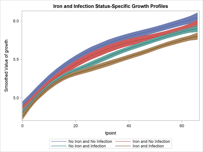
Next, the smoothed estimate of trend (growth) is graphically studied. The following DATA step prepares the data for the grouped plots of smoothed_growth by merging For1 with the input data set Cows. As before, the reason is merely to include ironInf (the grouping variable).

data For1;
    merge For1 Cows;
    by tpoint;
run;

The following statements produce the graphs of smoothed for the desired settings (since the grouping variable ironInf exactly corresponds to these settings). Once again, the plot in Output 27.4.9 clearly shows that the control group "No Iron and No Infection" has the best growth profile, while the worst growth profile is for the group "Iron and Infection." However, unlike the first model, the profile curves are not merely shifted versions of a common profile.

 proc sgplot data=For1 noautolegend;
    title 'Iron and Infection Status-Specific Growth Profiles';
     band x=tpoint lower=smoothed_lower_growth
       upper=smoothed_upper_growth / group=ironInf name="band";
     series  x=tpoint y=smoothed_growth / group=ironInf name="series";
     keylegend "series";
 run;

Output 27.4.9: Model 2: Growth Profile Comparison with 95% Confidence Bands

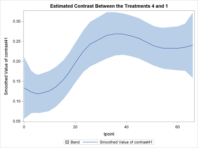
The following statements produce the plot of smoothed —contrast between the best and the worst growth profiles.

 proc sgplot data=For1;
    title "Estimated Contrast Between the Treatments 4 and 1 ";
     band x=tpoint lower=smoothed_lower_contrast41
        upper=smoothed_upper_contrast41;
     series x=tpoint y=smoothed_contrast41;
 run;

Output 27.4.10 shows that the growth pattern of the control group "No Iron and No Infection" consistently remains above the growth pattern of the treatment group "Iron and Infection."

Output 27.4.10: Estimated Contrast Between the Treatments 4 and 1 with 95% Confidence Bands