The SSM Procedure
-
Overview

- Getting Started
-
Syntax
-
DetailsState Space Model and NotationTypes of Sequence DataOverview of Model Specification SyntaxFiltering, Smoothing, Likelihood, and Structural Break DetectionEstimation of User-Specified Linear Combination of State ElementsContrasting PROC SSM with Other SAS Procedures Predefined Trend ModelsPredefined Structural ModelsCovariance ParameterizationMissing ValuesComputational IssuesDisplayed OutputODS Table NamesODS Graph NamesOUT= Data Set
-
ExamplesBivariate Basic Structural Model Panel Data: Random-Effects and Autoregressive ModelsBackcasting, Forecasting, and InterpolationLongitudinal Data: Smoothing of Repeated MeasuresA User-Defined Trend ModelModel with Multiple ARIMA ComponentsDynamic Factor ModelingDiagnostic Plots and Structural Break AnalysisLongitudinal Data: Variable Bandwidth SmoothingA Transfer Function Model for the Gas Furnace DataPanel Data: Dynamic Panel Model for the Cigar DataMultivariate Modeling: Long-Term Temperature TrendsBivariate Model: Sales of Mink and Muskrat FursFactor Model: Now-Casting the US EconomyLongitudinal Data: Lung Function Analysis
- References
The data for this example, taken from Givens and Hoeting (2005, chap. 11, Example 11.8), contain two variables, x and y. The variable y represents noisy evaluation of an unknown smooth function at x. The data are sorted by x.
 data Difficult;
 input x y;
 datalines;
 0.002 0.040
 0.011 0.009
 0.013 0.719
 0.016 0.199
 0.017 -0.409

   ... more lines ...
Output 27.9.1 shows the scatter plot of y against x that is generated by the following statements:
 proc sgplot data=Difficult;
    title "Scatter Plot of Y versus X";
    scatter x=x y=y ;
 run;
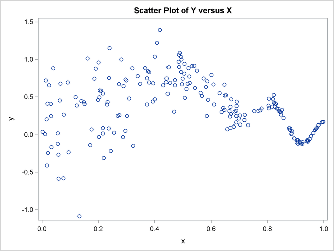
The plot clearly shows that the variance of y values varies considerably over the range of x values—the variance is larger for x values around 0.2 and gets increasingly smaller as the x values get closer to 1. Givens and Hoeting (2005) discuss the difficulties of extracting a smooth pattern from such data. Consider the following model for y:
where ![]() is a smooth trend component and
is a smooth trend component and ![]() is the observation noise with variance,
is the observation noise with variance, ![]() , which changes with
, which changes with x: ![]() . It is known (Durbin and Koopman, 2001, chap. 3, sect. 10 and sect. 11) that modeling the trend
. It is known (Durbin and Koopman, 2001, chap. 3, sect. 10 and sect. 11) that modeling the trend ![]() as a polynomial smoothing spline (for example, the way the growth curves are modeled in Example 27.4) and taking the variance function of the observation noise
as a polynomial smoothing spline (for example, the way the growth curves are modeled in Example 27.4) and taking the variance function of the observation noise ![]() a constant results in a trend estimate that can be termed a fixed-bandwidth-smoother. The optimal bandwidth turns out to
be a function of the signal-to-noise ratio: the ratio of the observation noise variance and the disturbance variance of the
trend component. On the other hand, allowing the variance function of the observation noise to change with the
a constant results in a trend estimate that can be termed a fixed-bandwidth-smoother. The optimal bandwidth turns out to
be a function of the signal-to-noise ratio: the ratio of the observation noise variance and the disturbance variance of the
trend component. On the other hand, allowing the variance function of the observation noise to change with the x values results in a trend estimate that can be termed a variable-bandwidth-smoother. The rest of this example shows how to
use the SSM procedure to create a data-dependent variance function ![]() and to extract the associated (variable-bandwidth) smooth trend from such data. Suppose that the (unknown) variance function
and to extract the associated (variable-bandwidth) smooth trend from such data. Suppose that the (unknown) variance function
![]() can be approximated as
can be approximated as
where ![]() are unknown parameters and
are unknown parameters and ![]() , are the full set of cubic spline basis functions (B-splines) with four evenly spaced internal knots between the range of
, are the full set of cubic spline basis functions (B-splines) with four evenly spaced internal knots between the range of
x values—essentially, four equispaced points between 0.0 and 1.0. Note that the number of basis functions in the full set,
7, is the sum of the number of internal knots, 4, and the degree of the polynomial, 3. The following statements create a data
set, Combined, that contains the variables x and y, along with the desired spline basis functions (col1–col7) that are created by using the BSPLINE function in PROC IML:
 proc iml;
    use difficult;
    /* read x and y from difficult into temp */
    read all var _num_ into temp;
    x = temp[,1];
    /* generate B-spline basis for a cubic spline
       with 4 evenly spaced internal knots in the x-range */
    bsp = bspline(x, 2, ., 4);
    Combined = temp || bsp;
    /* create a merged data set with x, y, and
       spline basis columns                    */
    create Combined var {x y col1 col2 col3 col4 col5 col6 col7};
    append from Combined;
 quit;
The following statements specify and fit the desired model to the data:
 proc ssm data=Combined opt(tech=dbldog);
    id x;
    /* parameters needed to define h(x) */
    parms v1-v7;
    /* defining h(x) */
    var = exp(v1*col1 + v2*col2 + v3*col3 + v4*col4
       + v5*col5 + v6*col6 + v7*col7);
    /* defining the polynomial spline trend */
    trend trend(ps(2));
    /* defining the observation noise with variance h(x) */
    irregular wn variance=var;
    model y = trend wn;
    output out=For pdv;
 run;
Output 27.9.2 shows the estimates of ![]() , and Output 27.9.3 shows the estimate of the disturbance variance associated with the polynomial spline trend that is specified in the TREND
statement.
, and Output 27.9.3 shows the estimate of the disturbance variance associated with the polynomial spline trend that is specified in the TREND
statement.
The following statements produce a plot, shown in Output 27.9.4, of the fitted trend with 95% confidence band:
 proc sgplot data=For;
    title "Variable Bandwidth Smoothing Spline";
    band x=x lower=smoothed_lower_trend
       upper=smoothed_upper_trend ;
    series x=x y=smoothed_trend;
    scatter x=x y=y;
 run;
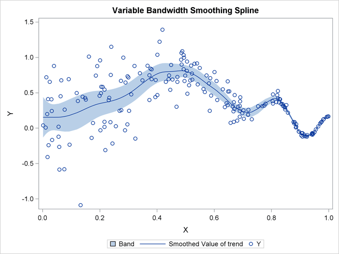
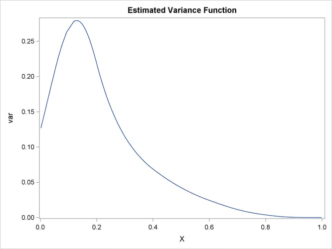
Clearly the fitted curve tracks the data quite well. Lastly, Output 27.9.5 (produced by using the following statements) shows the estimated variance function ![]() .
.
 proc sgplot data=For;
    title "Estimated Variance Function";
    series x=x y=var;
 run;
As expected, the curve attains its peak at an x value around 0.18 and decays to nearly 0 as x values reach 1.0.