The SSM Procedure
-
Overview

- Getting Started
-
Syntax
-
DetailsState Space Model and NotationTypes of Sequence DataOverview of Model Specification SyntaxFiltering, Smoothing, Likelihood, and Structural Break DetectionEstimation of User-Specified Linear Combination of State ElementsContrasting PROC SSM with Other SAS Procedures Predefined Trend ModelsPredefined Structural ModelsCovariance ParameterizationMissing ValuesComputational IssuesDisplayed OutputODS Table NamesODS Graph NamesOUT= Data Set
-
ExamplesBivariate Basic Structural Model Panel Data: Random-Effects and Autoregressive ModelsBackcasting, Forecasting, and InterpolationLongitudinal Data: Smoothing of Repeated MeasuresA User-Defined Trend ModelModel with Multiple ARIMA ComponentsDynamic Factor ModelingDiagnostic Plots and Structural Break AnalysisLongitudinal Data: Variable Bandwidth SmoothingA Transfer Function Model for the Gas Furnace DataPanel Data: Dynamic Panel Model for the Cigar DataMultivariate Modeling: Long-Term Temperature TrendsBivariate Model: Sales of Mink and Muskrat FursFactor Model: Now-Casting the US EconomyLongitudinal Data: Lung Function Analysis
- References
A well-known business conditions index, the Aruoba-Diebold-Scotti (ADS) business conditions index, is designed to track real
business conditions at high frequency (for more information about this index, see http://www.philadelphiafed.org/research-and-data/real-time-center/business-conditions-index/). Its underlying (seasonally adjusted) economic indicators (weekly initial jobless claims, monthly payroll employment, industrial
production, personal income less transfer payments, manufacturing and trade sales, and quarterly real GDP) blend high- and
low-frequency information with stock and flow data. The ADS index is based on a rather elaborate state space model that takes
into account the stock and flow nature of the underlying economic indicators. To simplify the illustration, this example uses
the same economic indicators to develop a similar index by using a simpler factor model. You can also use PROC SSM to carry
out the more elaborate modeling that underlies the ADS index. All these economic indicators are freely available from the
Federal Reserve Economic Data (FRED). You can access these data by using the SASEFRED interface engine; see Chapter 39: The SASEFRED Interface Engine. The names of analysis variables and the relevant information that is needed for using the SASEFRED engine to obtain these
data are shown in Table 27.11. All variables are transformed versions of the original series: all, except l_icsa, are both logged and differenced; l_icsa is only logged. The input data set for the analysis, named econ, is formed by merging these six series of different frequencies. This merging is done by treating them as daily series that
have missing values on the days when the series values are not available—for example, ld_pinc is nonmissing only for the first day of the month. The econ data set contains one more variable, recession, which is an indicator variable for the recessionary periods. This time series is an interpretation of the US Business Cycle
Expansions and Contractions data that are provided by the National Bureau of Economic Research (NBER) at http://www.nber.org/cycles/cyclesmain.html (also see http://research.stlouisfed.org/fred2/series/USRECDM). The variable recession is not used in modeling. It is used later to demonstrate the adequacy of the activity index that is created in this example.
Table 27.11: Analysis Variables and Their FRED IDs
|
Name |
FRED ID |
Frequency |
Description |
|---|---|---|---|
|
ld_payemp |
PAYEMS |
Monthly |
Payroll employment |
|
ld_pinc |
W875RX1 |
Monthly |
Real personal income excluding current transfer receipts |
|
ld_mnfctr |
CMRMTSPL |
Monthly |
Real manufacturing and trade industries sales |
|
ld_indpro |
INDPRO |
Monthly |
Industrial production index |
|
ld_gdp |
GDPC1 |
Quarterly |
Real GDP |
|
l_icsa |
ICSA |
Weekly |
Initial jobless claims |
For easier model description, the variables ld_payemp to ld_gdp are also denoted as ![]() to
to ![]() , and the variable
, and the variable l_icsa is denoted as ![]() . Using this notation, the following model is postulated for the six daily time series:
. Using this notation, the following model is postulated for the six daily time series:
A justification for this model is based on the following observations:
-
The five time series
 to
to  are logged and differenced versions of the underlying economic variables. Their plots (not shown here) show them to be hovering
around a constant level, with some periods of deviation from this level. The plot of the sixth series,
are logged and differenced versions of the underlying economic variables. Their plots (not shown here) show them to be hovering
around a constant level, with some periods of deviation from this level. The plot of the sixth series,  , which is logged but not differenced, shows a pronounced nonstationary pattern.
-
All these series can be considered as proxies, possibly noisy, for the national economic activity. It is therefore reasonable to assume that a model for each of them will contain a common component, appropriately weighted, that is associated with the economic activity. In the current model this common component, named
 , is modeled as an integrated random walk. For to , the only other terms in the model are the respective intercepts,
  , and the random disturbances,
  . Because shows a pronounced nonstationary pattern, its model includes an additional term,
  , which is also modeled as an integrated random walk. For identifiability purposes, the initial condition for is taken to be 0. For the same reason,
  , the coefficient of in the model for is taken to be 1.
-
The underlying economic variables of the five time series
to are positively correlated with the economic activity—for example, payroll employment is expected to increase with increased
economic activity. On the other hand, , which is associated with the initial jobless claims, is negatively correlated with the economic activity. This means that,
with taken to be 1, the estimates of  are expected to be positive and the estimate of
  is expected to be negative. In the factor modeling terminology, is called a factor and
  are called the associated factor loadings.
The following statements show you how to specify this model in the SSM procedure:
 ods output NamedParameterEstimates = named;
 proc ssm data=econ opt(tech=activeset);
   id date interval=day;
   parms beta2-beta6;
   parms lv1-lv8;
   avar = exp(lv7);
   wnv1 = exp(lv1);  wnv2 = exp(lv2);
   wnv3 = exp(lv3);  wnv4 = exp(lv4);
   wnv5 = exp(lv5);  wnv6 = exp(lv6);
   tvar = exp(lv8);
   zero = 0;

    /* --- start of model spec ----*/
   state latent(2) t(g)=(1 1 0 1) cov(d)=(zero avar);
   comp c1 = latent[1];
   comp c2 = (beta2)*latent[1];
   comp c3 = (beta3)*latent[1];
   comp c4 = (beta4)*latent[1];
   comp c5 = (beta5)*latent[1];
   comp c6 = (beta6)*latent[1];

   irregular w1 variance=wnv1;
   int1 = 1;
   model ld_payemp = int1 c1 w1;

   irregular w2 variance=wnv2;
   int2 = 1;
   model ld_pinc = int2 c2 w2;

   irregular w3 variance=wnv3;
   int3 = 1;
   model ld_mnfctr = int3 c3 w3;

   irregular w4 variance=wnv4;
   int4 = 1;
   model ld_indpro = int4 c4 w4;

   irregular w5 variance=wnv5;
   int5 = 1;
   model ld_gdp = int5 c5 w5;

   irregular w6 variance=wnv6 ;
   trend t_icsa(ll) levelvar=0 slopevar=tvar;
   model l_icsa = c6 t_icsa w6;
   /* ---model spec done----*/

   eval icsaPattern = c6 + t_icsa;
   /*--index is a scaled version of the common factor--*/
   eval Index = 1000*c1;
   comp slope = latent[2];
   eval IndexSlope = 1000*slope;
   /*--just so recession is output to the output data set--*/
   rec = recession;
   output out=forecast1 press pdv;
  run;
A few comments about the program:
-
If the model and data are in reasonable accord, the default likelihood optimization settings work in most situations. However, in some cases the likelihood optimization process needs additional customization. Some experimentation with alternative optimization techniques and different parameterization of the model parameters can help. This example turns out to be one such case. Here the optimization technique ACTIVESET (
opt(tech=activeset)) seems to work better. In addition, the variances of all the disturbance terms in the model are parameterized in the exponential scale. -
The two-dimensional state that is associated with
is named latent, and (the first element of latent) itself is namedc1. Note that the second element oflatentcorresponds to the slope of. The components c2toc6correspond to for
for  .
.
-
The desired business index, named
index, is a scaled version of (eval Index = 1000*c1;). This scaling is done purely for ease of display—the scaled values turn out to be in the range of –6.0 to 5.0. Another component, namedIndexSlope, contains the slope ofindex, which is also a quantity of interest.
Output 27.14.1 shows the estimated factor loadings. They are statistically significant and their signs are consistent.
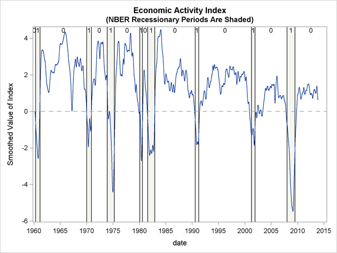
Output 27.14.2 shows the plot of the smoothed index. Note that it coheres quite well with the NBER recessionary periods. In Aruoba, Diebold,
and Scotti (2009, sec. 4.4) the features of an earlier version of the ADS index are discussed in detail. Similar comments apply to this indicator
also.
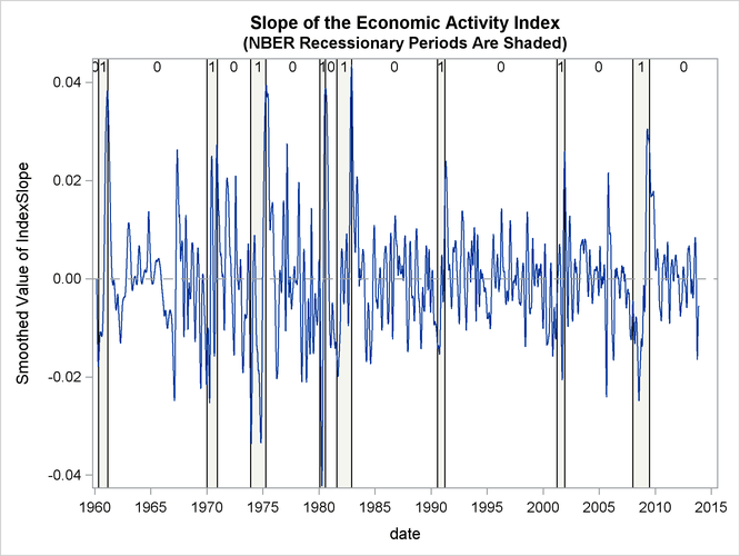
Finally, Output 27.14.3 shows the plot of the slope of the index, which gives an idea of the direction of the economic activity.