The SSM Procedure
-
Overview

- Getting Started
-
Syntax
-
DetailsState Space Model and NotationTypes of Sequence DataOverview of Model Specification SyntaxFiltering, Smoothing, Likelihood, and Structural Break DetectionEstimation of User-Specified Linear Combination of State ElementsContrasting PROC SSM with Other SAS Procedures Predefined Trend ModelsPredefined Structural ModelsCovariance ParameterizationMissing ValuesComputational IssuesDisplayed OutputODS Table NamesODS Graph NamesOUT= Data Set
-
ExamplesBivariate Basic Structural Model Panel Data: Random-Effects and Autoregressive ModelsBackcasting, Forecasting, and InterpolationLongitudinal Data: Smoothing of Repeated MeasuresA User-Defined Trend ModelModel with Multiple ARIMA ComponentsDynamic Factor ModelingDiagnostic Plots and Structural Break AnalysisLongitudinal Data: Variable Bandwidth SmoothingA Transfer Function Model for the Gas Furnace DataPanel Data: Dynamic Panel Model for the Cigar DataMultivariate Modeling: Long-Term Temperature TrendsBivariate Model: Sales of Mink and Muskrat FursFactor Model: Now-Casting the US EconomyLongitudinal Data: Lung Function Analysis
- References
This example illustrates how you can use the SSM procedure to analyze a bivariate time series. The following data set contains
two variables, f_KSI and r_KSI, which are measured quarterly, starting the first quarter of 1969. The variable f_KSI represents the quarterly average of the log of the monthly totals of the front-seat passengers killed or seriously injured
during the car accidents, and r_KSI represents a similar number for the rear-seat passengers. The data set has been extended at the end with eight missing values,
which represent four quarters, to cause the SSM procedure to produce model forecasts for this span.
data seatBelt;
input f_KSI r_KSI @@;
label f_KSI = "Front Seat Passengers Injured--log scale";
label r_KSI = "Rear Seat Passengers Injured--log scale";
date = intnx( 'quarter', '1jan1969'd, _n_-1 );
format date YYQS.;
datalines;
    6.72417 5.64654  6.81728 6.06123  6.92382 6.18190
    6.92375 6.07763  6.84975 5.78544  6.81836 6.04644
    7.00942 6.30167  7.09329 6.14476  6.78554 5.78212
    6.86323 6.09520  6.99369 6.29507  6.98344 6.06194
    6.81499 5.81249  6.92997 6.10534  6.96356 6.21298
    7.02296 6.15261  6.76466 5.77967  6.95563 6.18993
    7.02016 6.40524  6.87849 6.06308  6.55966 5.66084
    6.73627 6.02395  6.91553 6.25736  6.83576 6.03535
    6.52075 5.76028  6.59860 5.91208  6.70597 6.08029
    6.75110 5.98833  6.53117 5.67676  6.52718 5.90572
    6.65963 6.01003  6.76869 5.93226  6.44483 5.55616
    6.62063 5.82533  6.72938 6.04531  6.82182 5.98277
    6.64134 5.76540  6.66762 5.91378  6.83524 6.13387
    6.81594 5.97907  6.60761 5.66838  6.62985 5.88151
    6.76963 6.06895  6.79927 6.01991  6.52728 5.69113
    6.60666 5.92841  6.72242 6.03111  6.76228 5.93898
    6.54290 5.72538  6.62469 5.92028  6.73415 6.11880
    6.74094 5.98009  6.46418 5.63517  6.61537 5.96040
    6.76185 6.15613  6.79546 6.04152  6.21529 5.70139
    6.27565 5.92508  6.40771 6.13903  6.37293 5.96883
    6.16445 5.77021  6.31242 6.05267  6.44414 6.15806
    6.53678 6.13404 . . . . . . . .
run;
These data have been analyzed in Durbin and Koopman (2001, chap. 9, sec. 3). The analysis presented here is similar. To simplify the illustration, the monthly data have been converted to quarterly data and two predictors (the number of kilometers traveled and the real price of petrol) are excluded from the analysis. You can also use PROC SSM to carry out the more elaborate analysis in Durbin and Koopman (2001).
One of the original reasons for studying these data was to assess the effect on f_KSI of the enactment of a seat-belt law in February 1983 that compelled the front seat passengers to wear seat belts. A simple
graphical inspection of the data (not shown here) reveals that f_KSI and r_KSI do not show a pronounced upward or downward trend but do show seasonal variation, and that these two series seem to move
together. Additional inspection also shows that the seasonal effect is relatively stable throughout the data span. These considerations
suggest the following model for ![]() = (
= (f_KSI, r_KSI):
All the terms on the right-hand side of this equation are assumed to be statistically independent. These terms are as follows:
-
The predictor
 (defined as
 Q1_83_Shiftlater in the program) denotes a variable that is 0 before the first quarter of 1983, and 1 thereafter. is supposed to affect only f_KSI(the first element of ); it represents the enactment of the seat-belt law of 1983.
-
 denotes a bivariate random walk. It is supposed to capture the slowly changing level of the vector
  . To capture the fact that
 f_KSIandr_KSImove together (that is, they are co-integrated), the covariance of the disturbance term of this random walk is assumed to be of lower than full rank. -
 denotes a bivariate trigonometric seasonal term. In this model, it is taken to be fixed (that is, the seasonal effects do
not change over time).
denotes a bivariate trigonometric seasonal term. In this model, it is taken to be fixed (that is, the seasonal effects do
not change over time).
-
 denotes a bivariate white noise term, which captures the residual variation that is unexplained by the other terms in the
model.
denotes a bivariate white noise term, which captures the residual variation that is unexplained by the other terms in the
model.
The preceding model is an example of a (bivariate) basic structural model (BSM). The following statements specify and fit
this model to f_KSI and r_KSI:
 proc ssm data=seatBelt stateinfo;
    id date interval=quarter;
    Q1_83_Shift = (date >= '1jan1983'd);
    state error(2) type=WN cov(g) print=cov;
    component wn1 = error[1];
    component wn2 = error[2];
    state level(2) type=RW cov(rank=1) print=cov;
    component rw1 = level[1];
    component rw2 = level[2];
    state season(2) type=season(length=4);
    component s1 = season[1];
    component s2 = season[2];
    model f_KSI = Q1_83_Shift rw1 s1  wn1 / print=(smooth);
    model r_KSI = rw2 s2 wn2;
    eval f_KSI_sa = rw1 + Q1_83_Shift;
    output out=For1;
 run;
The PROC SSM statement specifies the input data set, seatBelt. The use of the STATEINFO option in the PROC SSM statement produces additional information about the model state vector and
its diffuse initial state. The optional ID statement specifies an index variable, date. The INTERVAL=QUARTER option in the ID statement indicates that the measurements were collected on a quarterly basis. Next,
a programming statement defines Q1_83_Shift, the predictor that represents the enactment of the seat-belt law of 1983. It is used later in the MODEL statement for f_KSI. Separate STATE statements specify the terms ![]() ,
, ![]() , and
, and ![]() because they are statistically independent. Each model that governs them (white noise for
because they are statistically independent. Each model that governs them (white noise for ![]() , random walk for
, random walk for ![]() , and trigonometric seasonal for
, and trigonometric seasonal for ![]() ) can be specified by using the TYPE= option of the STATE statement. When you use the TYPE= option, you can use the COV option
to specify the information about the disturbance covariance in the state transition equation. The other details, such as the
transition matrix specification and the specification of
) can be specified by using the TYPE= option of the STATE statement. When you use the TYPE= option, you can use the COV option
to specify the information about the disturbance covariance in the state transition equation. The other details, such as the
transition matrix specification and the specification of ![]() in the initial condition, are inferred from the TYPE= option. The use of PRINT=COV in the STATE statement causes the estimated
disturbance covariance to be printed. For
in the initial condition, are inferred from the TYPE= option. The use of PRINT=COV in the STATE statement causes the estimated
disturbance covariance to be printed. For ![]() (a white noise),
(a white noise), ![]() is zero and
is zero and ![]() for all
for all ![]() , where
, where ![]() is specified by the COV option. For
is specified by the COV option. For ![]() and
and ![]() the initial condition is fully diffuse—that is,
the initial condition is fully diffuse—that is, ![]() is an identity matrix of appropriate order and
is an identity matrix of appropriate order and ![]() . The total diffuse dimension of this model,
. The total diffuse dimension of this model, ![]() , is
, is ![]() as a result of one predictor,
as a result of one predictor, Q1_83_Shift, and two fully diffuse state subsections, ![]() and
and ![]() . The components in the model are defined by suitable linear combinations of these different state subsections. The program
statements define the model as follows:
. The components in the model are defined by suitable linear combinations of these different state subsections. The program
statements define the model as follows:
-
state error(2) type=WN cov(g);defines as a two-dimensional white noise, named
 error, with the covariance of general form. Then two COMPONENT statements definewn1andwn2as the first and second elements oferror, respectively. -
state level(2) type=RW cov(rank=1);defines as a two-dimensional random walk, named level, with covariance of general form whose rank is restricted to 1. Then two COMPONENT statements definerw1andrw2as the first and second elements oflevel, respectively. -
state season(2) type=season(length=4);defines as a two-dimensional trigonometric seasonal of season length 4, named
 season, with zero covariance—signified by the absence of the COV option. Then two COMPONENT statements defines1ands2as appropriate linear combinations ofseasonso thats1represents the seasonal forf_KSIands2represents the seasonal forr_KSI. Because TYPE=SEASON in the STATE statement, the COMPONENT statement appropriately interpretscomponent s1 = season[1];ass1being a dot product: . See the section Multivariate Season for more information.
-
model f_KSI = Q1_83_Shift rw1 s1 wn1;defines the model forf_KSI, andmodel r_KSI = rw2 s2 wn2;defines the model forr_KSI.
The SSM procedure fits the model and reports the parameter estimates, their approximate standard errors, and the likelihood-based
goodness-of-fit measures by default. In order to output the one-step-ahead and full-sample estimates of the components in
the model, you can either use the PRINT= options in the MODEL statement and the respective COMPONENT statements or you can
specify an output data set in the OUTPUT statement. In addition, you can use the EVAL statement to define specific linear
combinations of the underlying state that should also be estimated. The statement eval f_KSI_sa = rw1 + Q1_83_Shift; is an example of one such linear combination. It defines f_KSI_sa, a linear combination that represents the seasonal adjustment of f_KSI. The output data set, For1 (named in the OUTPUT statement) contains estimates of all the model components in addition to the estimate of f_KSI_sa.
The model summary table, shown in Output 27.1.1, provides basic model information, such as the dimension of the underlying state equation (![]() ), the diffuse dimension of the model (
), the diffuse dimension of the model (![]() ), and the number of parameters (5) in the model parameter vector
), and the number of parameters (5) in the model parameter vector ![]() .
.
Additional details about the role of different components in forming the model state and its diffuse initial condition are
shown in Output 27.1.2 and Output 27.1.3. They show that the 10-dimensional model state vector is made up of subsections that are associated with error and level (each of dimension 2) and season (of dimension 6). Similarly, the nine-dimensional diffuse vector in the initial condition is made up of subsections that
correspond to level, season, and the regression variable, Q1_83_Shift. Note that error does not contribute to the diffuse initial vector because it has a fully nondiffuse initial state.
The index variable information is shown in Output 27.1.4.
Output 27.1.5 provides simple summary information about the response variables. It shows that f_KSI and r_KSI have four missing values each and no induced missing values because the predictor in the model, Q1_83_Shift, has no missing values.
The regression coefficient of Q1_83_Shift, shown in Output 27.1.6, is negative and is statistically significant. This is consistent with the expected drop in f_KSI after the enactment of the seat-belt law.
Output 27.1.7 shows the estimates of the elements of ![]() . The five parameters in
. The five parameters in ![]() correspond to unknown elements that are associated with the covariance matrices in the specifications of
correspond to unknown elements that are associated with the covariance matrices in the specifications of error and level. Whenever a covariance specification is of a general form and is not defined by a user-specified variable list, it is internally
parameterized as a product of its Cholesky root: ![]() . This ensures that the resulting covariance is positive semidefinite. The Cholesky root is constrained to be lower triangular,
with positive diagonal elements. If rank constraints (such as the rank-one constraint on the covariance in the specification
of
. This ensures that the resulting covariance is positive semidefinite. The Cholesky root is constrained to be lower triangular,
with positive diagonal elements. If rank constraints (such as the rank-one constraint on the covariance in the specification
of level) are imposed, the number of free parameters in the Cholesky factor is reduced appropriately. See the section Covariance Parameterization for more information. In view of these considerations, the five parameters in ![]() are a result of three parameters from the Cholesky root of
are a result of three parameters from the Cholesky root of error and two parameters that are associated with the Cholesky root of level.
Output 27.1.7: Parameter Estimates
| Model Parameter Estimates | ||||
|---|---|---|---|---|
| Component | Type | Parameter | Estimate | Standard Error |
| error | Disturbance Covariance | RootCov[1, 1] | 0.0361 | 0.00736 |
| error | Disturbance Covariance | RootCov[2, 1] | 0.0338 | 0.01131 |
| error | Disturbance Covariance | RootCov[2, 2] | 0.0462 | 0.00470 |
| level | Disturbance Covariance | RootCov[1, 1] | 0.0375 | 0.00843 |
| level | Disturbance Covariance | RootCov[2, 1] | 0.0223 | 0.00569 |
Output 27.1.8 shows the resulting covariance estimate of error after multiplying the Cholesky factors.
Similarly, Output 27.1.9 shows the covariance estimate of level disturbance. Note that because of the rank-one constraint, the determinant of this matrix is 0.
Output 27.1.10 shows the likelihood computation summary. This table is produced by using the fitted model to carry out the filtering operation on the data. See the section Likelihood Computation and Model Fitting Phase for more information.
The output data set, For1, specified in the OUTPUT statement contains one-step-ahead and full-sample estimates of all the model components and the
user-specified components (defined by the EVAL statement). Their standard errors and the upper and lower confidence limits
(by default, 95%) are also produced.
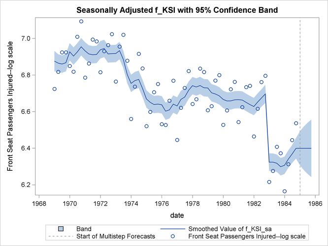
The following statements use the For1 data set to produce a time series plot of the seasonally adjusted f_KSI:
 proc sgplot data=For1;
    title "Seasonally Adjusted f_KSI with 95% Confidence Band";
    band x=date lower=smoothed_lower_f_KSI_sa
       upper=smoothed_upper_f_KSI_sa ;
    series x=date y=smoothed_f_KSI_sa;
    refline '1jan1985'd / axis=x lineattrs=(pattern=shortdash)
       LEGENDLABEL= "Start of Multistep Forecasts"
       name="Forecast Reference Line";
    scatter x=date y=f_KSI ;
 run;
The generated plot is shown in Output 27.1.11.