The SSM Procedure
-
Overview

- Getting Started
-
Syntax
-
DetailsState Space Model and NotationTypes of Sequence DataOverview of Model Specification SyntaxFiltering, Smoothing, Likelihood, and Structural Break DetectionEstimation of User-Specified Linear Combination of State ElementsContrasting PROC SSM with Other SAS Procedures Predefined Trend ModelsPredefined Structural ModelsCovariance ParameterizationMissing ValuesComputational IssuesDisplayed OutputODS Table NamesODS Graph NamesOUT= Data Set
-
ExamplesBivariate Basic Structural Model Panel Data: Random-Effects and Autoregressive ModelsBackcasting, Forecasting, and InterpolationLongitudinal Data: Smoothing of Repeated MeasuresA User-Defined Trend ModelModel with Multiple ARIMA ComponentsDynamic Factor ModelingDiagnostic Plots and Structural Break AnalysisLongitudinal Data: Variable Bandwidth SmoothingA Transfer Function Model for the Gas Furnace DataPanel Data: Dynamic Panel Model for the Cigar DataMultivariate Modeling: Long-Term Temperature TrendsBivariate Model: Sales of Mink and Muskrat FursFactor Model: Now-Casting the US EconomyLongitudinal Data: Lung Function Analysis
- References
This example shows how to specify a continuous-time trend model discussed in Harvey (1989, chap. 9, sec. 9.2.1). This model is not one of the predefined trend models in the SSM procedure. The system matrices that govern the two-dimensional state of this model are
where ![]() denotes the difference between the successive time points, and the parameters
denotes the difference between the successive time points, and the parameters ![]() and
and ![]() are called the level variance and the slope variance, respectively. The initial condition is fully diffuse. The trend component
corresponds to the first element of this state vector. The second element of the state vector corresponds to the slope of
this trend component. This model reduces to the polynomial spline model of order 2 if the level variance
are called the level variance and the slope variance, respectively. The initial condition is fully diffuse. The trend component
corresponds to the first element of this state vector. The second element of the state vector corresponds to the slope of
this trend component. This model reduces to the polynomial spline model of order 2 if the level variance ![]() . See the section Polynomial Spline Trend.
. See the section Polynomial Spline Trend.
The following statements specify a trend-plus-noise model to model the growth of cows in the previous example ( Example 27.4). The only cows that are considered are the ones that received iron and are infected.
 proc ssm data=Cows;
    where iron=1 and infection=1;
    id tpoint;
    parms var1 var2 / lower=(1.e-8 1.e-8);
    array tMat{2,2};
    tMat[1,1] = 1;
    tMat[2,2] = 1;
    tMat[1,2] = _ID_DELTA_;
    array covMat{2,2};
    covMat[1,1] = var1*_ID_DELTA_ + var2*_ID_DELTA_**3/3;
    covMat[1,2] = var2*_ID_DELTA_**2/2;
    covMat[2,1] = covMat[1,2] ;
    covMat[2,2] = var2*_ID_DELTA_;
    state harveyLL(2) T(g)=(tMat) cov(g)=(covMat) a1(2);
    component trend = harveyLL[1];
    component slope = harveyLL[2];
    irregular wn;
    model  weight = trend  wn;
    output out=for;
 run;
The program is easy to follow. The PARMS statement declares var1 and var2 as positive parameters, which correspond to ![]() and
and ![]() , respectively. The programming statements define arrays
, respectively. The programming statements define arrays tMat and covMat, which later become the matrices ![]() and
and ![]() , respectively. Note that the element
, respectively. Note that the element tMat[2,1] is left unassigned, since it is a structural zero of ![]() (see the section Sparse Transition Matrix Specification for more information). Recall that the predefined variable
(see the section Sparse Transition Matrix Specification for more information). Recall that the predefined variable _ID_DELTA_ contains the value of ![]() , which is needed for defining the elements of
, which is needed for defining the elements of ![]() and
and ![]() (see the section ID Statement). The STATE statement defines the trend state vector,
(see the section ID Statement). The STATE statement defines the trend state vector, harveyLL, and the COMPONENT statement defines the trend component, trend, by selecting the first element of harveyLL. An additional COMPONENT statement defines the slope component, slope, as the second element of harveyLL. The slope component (which represents the cow’s growth rate) is not part of the observation equation; it is specified so that its estimate
is output to For (the OUT= data set specified in the OUTPUT statement). The IRREGULAR statement defines the observation noise, and the MODEL
statement defines the trend-plus-noise model.
The estimates of var1 and var2 are shown in Output 27.5.1. It shows that the estimate of the level variance is nearly 0, implying that the fitted trend model is identical to the polynomial
spline trend of order 2.
The estimate of the noise variance is shown in Output 27.5.2.
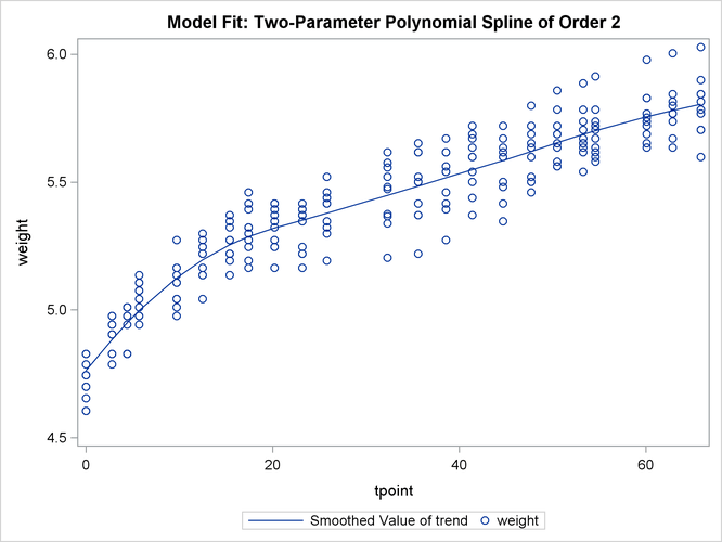
The following statements produce the plot of the fit of this trend model (shown in Output 27.5.3).
 proc sgplot data=For;
     title "Model Fit: Two-Parameter Polynomial Spline of Order 2";
     series x=tpoint y=smoothed_trend;
     scatter x=tpoint y=weight;
 run;
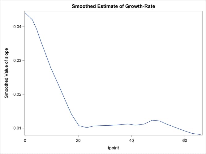
The following statements produce the plot of the estimate of the slope component (shown in Output 27.5.4). This plot complements the preceding plot of trend; it shows the pattern of decline in the growth rate as the animals age.
 proc sgplot data=For;
     title "Smoothed Estimate of Growth-Rate";
     series x=tpoint y=smoothed_slope;
 run;