The SSM Procedure
-
Overview

- Getting Started
-
Syntax
-
DetailsState Space Model and NotationTypes of Sequence DataOverview of Model Specification SyntaxFiltering, Smoothing, Likelihood, and Structural Break DetectionEstimation of User-Specified Linear Combination of State ElementsContrasting PROC SSM with Other SAS Procedures Predefined Trend ModelsPredefined Structural ModelsCovariance ParameterizationMissing ValuesComputational IssuesDisplayed OutputODS Table NamesODS Graph NamesOUT= Data Set
-
ExamplesBivariate Basic Structural Model Panel Data: Random-Effects and Autoregressive ModelsBackcasting, Forecasting, and InterpolationLongitudinal Data: Smoothing of Repeated MeasuresA User-Defined Trend ModelModel with Multiple ARIMA ComponentsDynamic Factor ModelingDiagnostic Plots and Structural Break AnalysisLongitudinal Data: Variable Bandwidth SmoothingA Transfer Function Model for the Gas Furnace DataPanel Data: Dynamic Panel Model for the Cigar DataMultivariate Modeling: Long-Term Temperature TrendsBivariate Model: Sales of Mink and Muskrat FursFactor Model: Now-Casting the US EconomyLongitudinal Data: Lung Function Analysis
- References
The data for this example, which consist of 209 measurements of the lung function of an asthma patient, are analyzed in Wang (2013). The time series is measured mostly at two-hour time intervals but with irregular gaps. Wang (2013) fit a fourth-order continuous-time autoregressive model, CAR(4), to these data. The analysis results in a decomposition of the observed time series in three components:
-
a slowly varying trend pattern, which appears to have a slight downward drift
-
a diurnal component—a periodic pattern with a period of 24 hours
-
a residual component
As shown in Wang (2013), the continuous-time autoregressive models can be formulated as state space models. However, in general, the form of such
SSMs is quite complex. Consequently, specifying such a model by using the current SSM procedure syntax is impractical. On
the other hand, you can analyze these types of longitudinal data by using continuous-time structural models, which are easy
to specify in the SSM procedure. In this example, the lung function measurements, y, are modeled as
where ![]() is a simple linear time trend,
is a simple linear time trend, ![]() is a continuous-time stochastic cycle, and
is a continuous-time stochastic cycle, and ![]() is a Gaussian white noise sequence. Replacing the linear time trend with a more general time trend, such as a spline smoother,
does not seem to change the fit, because the estimated smoothing spline turns out to be almost perfectly linear.
is a Gaussian white noise sequence. Replacing the linear time trend with a more general time trend, such as a spline smoother,
does not seem to change the fit, because the estimated smoothing spline turns out to be almost perfectly linear.
The following statements show you how to specify this model in the SSM procedure:
proc ssm data=asth;
   id time;
   state s1(1) type=cycle(CT) cov(g);
   comp c1 = s1[1];
   intercept = 1;
   irregular wn;
   model y= intercept time c1 wn;
   output out=for1 press;
   eval pattern=intercept+time+c1;
run;
The continuous-time stochastic cycle, named c1, is defined by a pair of STATE and COMPONENT statements. The STATE statement defines s1 as a state subsection that is associated with a univariate, continuous-time cycle (signified by the use of type=cycle(CT)). The COMPONENT statement defines c1 as its first element.
Output 27.15.1 shows the estimated intercept and slope of the time trend. The estimated slope (only marginally significant) is negative,
which is consistent with the overall downward drift.
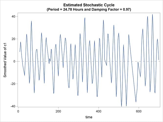
Output 27.15.2 shows the plot of the estimated cycle component, which has a period of 24.78 hours and a damping factor of 0.97. That is,
it is a nearly persistent diurnal cycle.
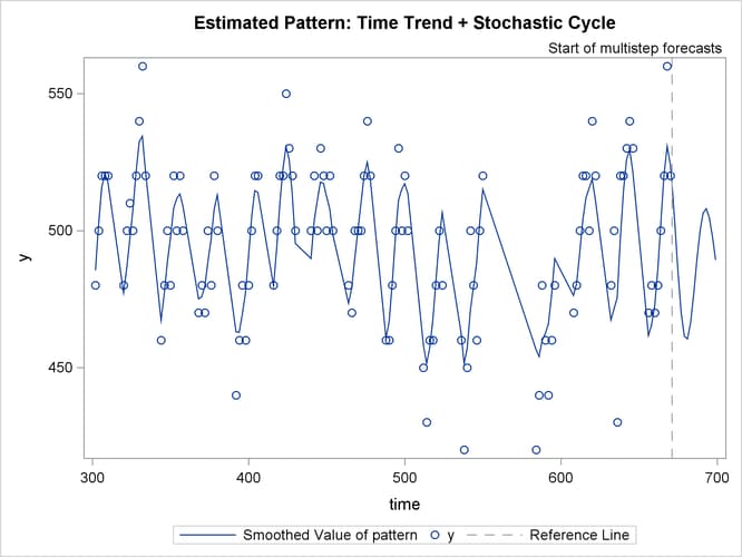
Output 27.15.3 shows the fit of the de-noised y values (![]() ). To reduce the clutter, only the second half of the data are plotted. The fit appears to be quite reasonable.
). To reduce the clutter, only the second half of the data are plotted. The fit appears to be quite reasonable.