The SSM Procedure
-
Overview

- Getting Started
-
Syntax
-
DetailsState Space Model and NotationTypes of Sequence DataOverview of Model Specification SyntaxFiltering, Smoothing, Likelihood, and Structural Break DetectionEstimation of User-Specified Linear Combination of State ElementsContrasting PROC SSM with Other SAS Procedures Predefined Trend ModelsPredefined Structural ModelsCovariance ParameterizationMissing ValuesComputational IssuesDisplayed OutputODS Table NamesODS Graph NamesOUT= Data Set
-
ExamplesBivariate Basic Structural Model Panel Data: Random-Effects and Autoregressive ModelsBackcasting, Forecasting, and InterpolationLongitudinal Data: Smoothing of Repeated MeasuresA User-Defined Trend ModelModel with Multiple ARIMA ComponentsDynamic Factor ModelingDiagnostic Plots and Structural Break AnalysisLongitudinal Data: Variable Bandwidth SmoothingA Transfer Function Model for the Gas Furnace DataPanel Data: Dynamic Panel Model for the Cigar DataMultivariate Modeling: Long-Term Temperature TrendsBivariate Model: Sales of Mink and Muskrat FursFactor Model: Now-Casting the US EconomyLongitudinal Data: Lung Function Analysis
- References
This example provides information about the diagnostic plots that the SSM procedure produces. In addition, a simple illustration of structural break analysis is also provided. The following plots are available in the SSM procedure:
-
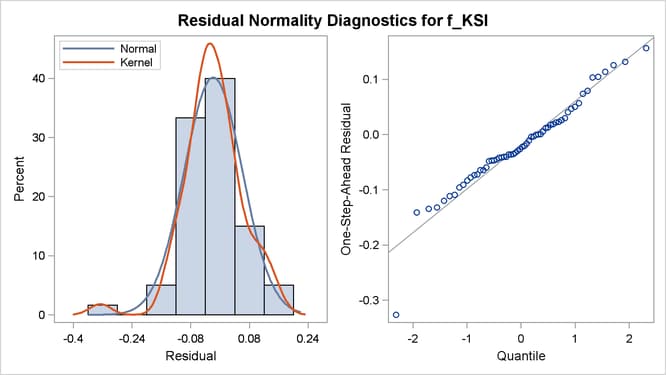
a panel of two plots—a histogram and a Q-Q plot—for the normality check of the one-step-ahead residuals
 . A separate panel is produced for each response variable.
-
a time series plot of standardized residuals, one per response variable
-
a panel of two plots—a histogram and a Q-Q plot—for the normality check of the prediction errors
 . A separate panel is produced for each response variable.
-
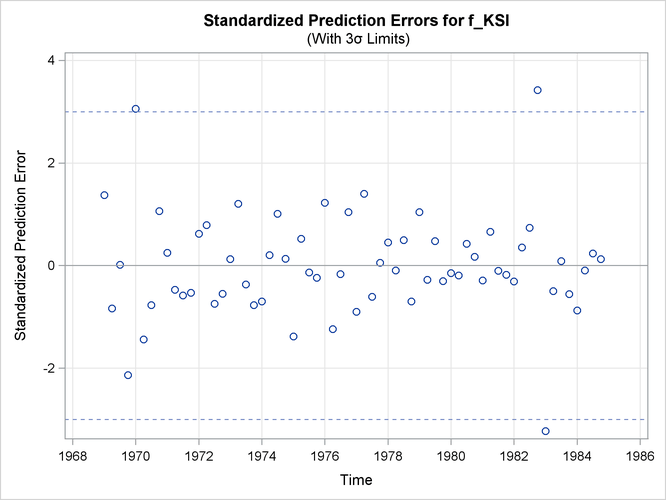
a time series plot of standardized prediction errors, one per response variable
-
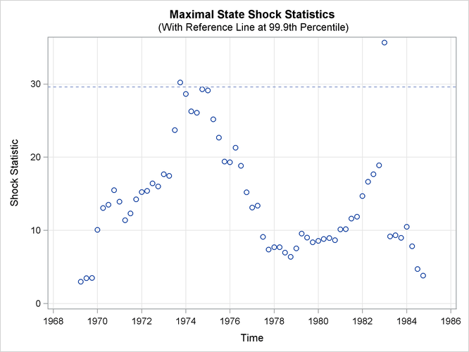
a time series plot of maximal state shock chi-square statistics
All these plots are used primarily for model diagnostics. In this example, the automobile seat-belt data that are discussed
in Example 27.1 are revisited. In Example 27.1, the question under consideration is whether the data show evidence of the effectiveness of the seat-belt law that was introduced
in the first quarter of 1983. An intervention variable, Q1_83_Shift, was used in the model to measure the effect of this law on the drivers and front-seat passengers who were killed or seriously
injured in car accidents (f_KSI). In the current example, the analysis of these data begins without the knowledge of this seat-belt law. In effect, the same
model is fitted without the use of the intervention variable Q1_83_Shift.
The following statements specify the model (without the intervention variable):
 proc ssm data=seatBelt optimizer(tech=interiorpoint) plots=all;
    id date interval=quarter;
    state error(2) type=WN cov(g);
    component wn1 = error[1];
    component wn2 = error[2];
    state level(2) type=RW cov(rank=1) checkbreak;
    component rw1 = level[1];
    component rw2 = level[2];
    state season(2) type=season(length=4);
    component s1 = season[1];
    component s2 = season[2];
    model f_KSI = rw1 s1  wn1;
    model r_KSI = rw2 s2 wn2;
 run;
The PLOTS=ALL option in the PROC SSM statement turns on all the plotting options. Because there are two response variables,
nine plots in total are produced: a separate set of four plots—two residual and two prediction error—is produced for f_KSI and r_KSI, and one maximal shock plot is produced. Only three of these plots are shown here. Output 27.8.1 shows the normality check for the one-step-ahead residuals for f_KSI. It shows some evidence of lack of normality.
Output 27.8.2 shows the time series plot of standardized prediction errors for f_KSI. It identifies some extreme observations (additive outliers): two near 1983 and one near 1970.
Output 27.8.3 shows the time series plot of maximal shock statistics. This plot can be very informative in showing the temporal locations
of the structural changes in the overall observation-generation process (treating the fitted model as the reference). It can
indicate locations of shifts in the process level or shifts in other characteristics, such as its slope. The precise nature
of the shift (whether the shift occurs in the level or in some other aspects) can be determined by using the CHECKBREAK option
in the appropriate STATE and TREND statements (as is done in the STATE statement in this example that defines the bivariate
state level). In this example, the maximal shock statistics plot indicates two locations—the last quarter of 1973 and the first quarter
of 1983—as likely locations for the structural breaks that are associated with the traffic accident process. These are indeed
reasonable findings, because the last quarter of 1973 (beginning in October 1973) is associated with the start of the oil
crisis that severely curtailed worldwide automobile traffic, and the first quarter of 1983 is associated with the introduction
of the seat-belt law that might have improved the safety of drivers and front-seat passengers. In addition, Output 27.8.4 shows the summary of most likely break locations for the bivariate state level. It identifies a break in the first element of level (which corresponds to the drivers and front-seat passengers) in the first quarter of 1983.
The following statements fit a revised model that accounts for the break in the first element of level by introducing a dummy variable, Q1_83_Pulse, in the state equation:
 ods output ElementStateBreakDetails=stateBreak;
 proc ssm data=seatBelt optimizer(tech=interiorpoint) plots=all;
    id date interval=quarter;
    Q1_83_Pulse = (date = '1jan1983'd);
    zero = 0;
    state error(2) type=WN cov(g);
    component wn1 = error[1];
    component wn2 = error[2];
    state level(2) type=RW cov(rank=1) W(g)=(Q1_83_Pulse zero)
        checkbreak print=breakdetail;
    component rw1 = level[1];
    component rw2 = level[2];
    state season(2) type=season(length=4);
    component s1 = season[1];
    component s2 = season[2];
    model f_KSI =  rw1 s1  wn1;
    model r_KSI = rw2 s2 wn2;
 run;
Note that using Q1_83_Pulse in the definition of level is equivalent to using Q1_83_Shift in the MODEL statement for f_KSI in Example 27.1. Output 27.8.5 shows the estimated change in the first element of the state level, which is the same as the estimated level shift shown in Output 27.1.6 (this is not surprising, because these two models are statistically equivalent).
In the preceding SSM procedure statements, the CHECKBREAK option is used along with the PRINT=BREAKDETAIL option, which produces
a table that contains the break statistics at every distinct time point (this table, in turn, is captured in the output data
set stateBreak for later use). Output 27.8.6 shows the time series plot of maximal shock statistics for this revised model. As expected, the plot no longer shows the
first quarter of 1983 as a structural break location. It continues to show the last quarter of 1973 as a structural break
location, because the fitted model does not try to explicitly account for this shift.

Note that the reference line in Output 27.8.3 is drawn at the 99.9th percentile, whereas the reference line in Output 27.8.6 is drawn at the 99th percentile. The reference line location in the maximal state shock chi-square statistics plot is based
on the points in the plot. A reference line is drawn at percentile 80, 90, 99, or 99.9 based on the largest maximal shock
statistic that is shown.
The detailed information in the data set stateBreak can be used to further investigate the possibility of significant breaks in the trend in and around 1973. The following statements
produce scatter plots for the break statistics for both the drivers and front passengers and the rear passengers (reference
lines are also drawn at –3 and 3 to check for extreme Z values):
 proc sgpanel data=stateBreak;
     panelby elementIndex;
     scatter x=time y=zValue;
     refline 3 / axis=y lineattrs=(pattern=shortdash) noclip;
     refline -3 / axis=y lineattrs=(pattern=shortdash) noclip;
 run;
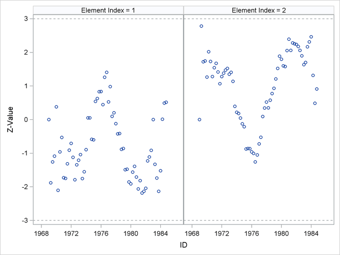
The resulting graph, shown in Output 27.8.7, shows possible breaks in the second element—rear side passengers—around 1969. In general, however, the evidence of breaks
in the elements of level is not very strong. This means that you must look elsewhere to explain the extreme point in Output 27.8.6.