The SSM Procedure
-
Overview

- Getting Started
-
Syntax
-
DetailsState Space Model and NotationTypes of Sequence DataOverview of Model Specification SyntaxFiltering, Smoothing, Likelihood, and Structural Break DetectionEstimation of User-Specified Linear Combination of State ElementsContrasting PROC SSM with Other SAS Procedures Predefined Trend ModelsPredefined Structural ModelsCovariance ParameterizationMissing ValuesComputational IssuesDisplayed OutputODS Table NamesODS Graph NamesOUT= Data Set
-
ExamplesBivariate Basic Structural Model Panel Data: Random-Effects and Autoregressive ModelsBackcasting, Forecasting, and InterpolationLongitudinal Data: Smoothing of Repeated MeasuresA User-Defined Trend ModelModel with Multiple ARIMA ComponentsDynamic Factor ModelingDiagnostic Plots and Structural Break AnalysisLongitudinal Data: Variable Bandwidth SmoothingA Transfer Function Model for the Gas Furnace DataPanel Data: Dynamic Panel Model for the Cigar DataMultivariate Modeling: Long-Term Temperature TrendsBivariate Model: Sales of Mink and Muskrat FursFactor Model: Now-Casting the US EconomyLongitudinal Data: Lung Function Analysis
- References
This example shows how you can fit the REGCOMPONENT models in Bell (2011) by using the SSM procedure. The following DATA step generates the data used in the last example of this article (Example
6: "Modeling a time series with a sampling error component"). The variable y in this data set contains monthly values of the VIP series (value of construction put in place), a U.S. Census Bureau publication
that measures the value of construction installed or erected at construction sites during a given month. The values of y are known to be contaminated with heterogeneous sampling errors; the variable hwt in the data set is a proxy for this sampling error in the log scale. The variable hwt is treated as a weight variable for the noise component in the model.
data Test;
  input y hwt;
  date = intnx('month', '01jan1997'd, _n_-1 );
  format date date.;
  logy = log(y);
  label logy = 'Log value of construction put in place';
  datalines;
115.2    0.042
110.4    0.042
111.5    0.067
127.9    0.122
150.0    0.129
149.5    0.135
139.5    0.152
144.6    0.168
176.0    0.173

   ... more lines ...
The article proposes the following model for the log VIP series:
where ![]() follows an ARIMA(0,1,1)
follows an ARIMA(0,1,1)![]() (0,1,1)
(0,1,1)![]() model and
model and ![]() is a zero-mean, AR(2) error process. The following statements specify this model for
is a zero-mean, AR(2) error process. The following statements specify this model for logy:
 proc ssm data=Test;
    id date interval=month;
    trend airlineTrend(arma(d=1 sd=1 q=1 sq=1 s=12));
    trend ar2Noise(arma(p=2)) cross=(hwt);
    model logy = airlineTrend ar2Noise;
    output outfor=For;
 run;
Output 27.6.1: Estimates of the ARIMA Components Model
| Model Parameter Estimates | ||||
|---|---|---|---|---|
| Component | Type | Parameter | Estimate | Standard Error |
| airlineTrend | ARMA Trend | Error Variance | 0.000642 | 0.00906 |
| airlineTrend | ARMA Trend | MA_1 | 0.251125 | 0.57239 |
| airlineTrend | ARMA Trend | SMA_1 | -0.710211 | 11.78177 |
| ar2Noise | ARMA Trend | Error Variance | 0.444514 | 0.14325 |
| ar2Noise | ARMA Trend | AR_1 | 0.481082 | 0.08027 |
| ar2Noise | ARMA Trend | AR_2 | 0.399923 | 0.21560 |
The ARIMA(0,1,1)![]() (0,1,1)
(0,1,1)![]() trend
trend ![]() is named
is named airlineTrend and the zero-mean, AR(2) error process ![]() is named
is named ar2Noise. See the TREND
statement for more information about the ARIMA notation. The estimates of model parameters are shown in Output 27.6.1. These estimates are different from the estimates given in the article; however, the estimated trend and noise series are
qualitatively similar. The article uses an estimation procedure that consists of a sequence of alternating steps in which
one subset of parameters is held fixed and the remaining parameters are estimated by MLE in each step. This process continues
until all the estimates stabilize. The SSM procedure estimates all the parameters simultaneously by MLE.
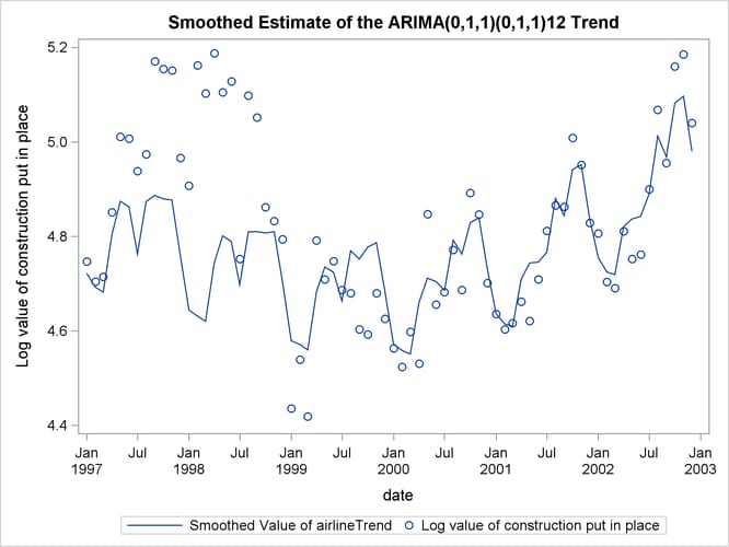
The following statements produce the plot of the estimate of the airlineTrend component (shown in Output 27.6.2). This plot is very similar to the trend plot shown in the article (the article plots are in the antilog scale).
 proc sgplot data=For;
     title "Smoothed Estimate of the ARIMA(0,1,1)(0,1,1)12 Trend";
     series x= date y=smoothed_airlineTrend;
     scatter x= date y=logy;
 run;
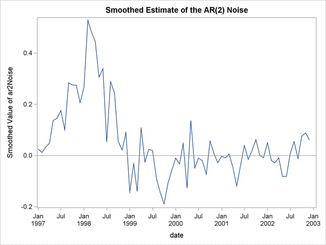
The following statements produce the plot of the estimate of the ar2Noise component (shown in Output 27.6.3). This plot is also very similar to the noise plot shown in the article (once again, the article plots are in the antilog
scale).
 proc sgplot data=For;
     title "Smoothed Estimate of the AR(2) Noise";
     series x= date y=smoothed_ar2Noise;
     refline 0;
 run;