The ARIMA Procedure
- Overview
-
Getting Started
 The Three Stages of ARIMA ModelingIdentification StageEstimation and Diagnostic Checking StageForecasting StageUsing ARIMA Procedure StatementsGeneral Notation for ARIMA ModelsStationarityDifferencingSubset, Seasonal, and Factored ARMA ModelsInput Variables and Regression with ARMA ErrorsIntervention Models and Interrupted Time SeriesRational Transfer Functions and Distributed Lag ModelsForecasting with Input VariablesData Requirements
 -
Syntax
-
DetailsThe Inverse Autocorrelation FunctionThe Partial Autocorrelation FunctionThe Cross-Correlation FunctionThe ESACF MethodThe MINIC MethodThe SCAN MethodStationarity TestsPrewhiteningIdentifying Transfer Function ModelsMissing Values and AutocorrelationsEstimation DetailsSpecifying Inputs and Transfer FunctionsInitial ValuesStationarity and InvertibilityNaming of Model ParametersMissing Values and Estimation and ForecastingForecasting DetailsForecasting Log Transformed DataSpecifying Series PeriodicityDetecting OutliersOUT= Data SetOUTCOV= Data SetOUTEST= Data SetOUTMODEL= SAS Data SetOUTSTAT= Data SetPrinted OutputODS Table NamesStatistical Graphics
-
Examples
- References
This example uses the Series J data from Box and Jenkins (1976). First, the input series X is modeled with a univariate ARMA model. Next, the dependent series Y is cross-correlated with the input series. Since a model has been fit to X, both Y and X are prewhitened by this model before the sample cross-correlations are computed. Next, a transfer function model is fit with
no structure on the noise term. The residuals from this model are analyzed; then, the full model, transfer function and noise,
is fit to the data.
The following statements read Input Gas Rate and Output CO![]() from a gas furnace. (Data values are not shown. The full example including data is in the SAS/ETS sample library.)
from a gas furnace. (Data values are not shown. The full example including data is in the SAS/ETS sample library.)
title1 'Gas Furnace Data';
title2 '(Box and Jenkins, Series J)';
data seriesj;
   input x y @@;
   label x = 'Input Gas Rate'
         y = 'Output CO2';
datalines;
-0.109  53.8  0.000  53.6  0.178  53.5  0.339  53.5

   ... more lines ...
The following statements produce Output 7.3.1 through Output 7.3.11:
proc arima data=seriesj;

   /*--- Look at the input process ----------------------------*/
   identify var=x;
   run;

   /*--- Fit a model for the input ----------------------------*/
   estimate p=3 plot;
   run;

   /*--- Cross-correlation of prewhitened series ---------------*/
   identify var=y crosscorr=(x) nlag=12;
   run;

   /*--- Fit a simple transfer function - look at residuals ---*/
   estimate input=( 3 $ (1,2)/(1) x );
   run;

   /*--- Final Model - look at residuals ----------------------*/
   estimate p=2 input=( 3 $ (1,2)/(1) x );
   run;

quit;
The results of the first IDENTIFY statement for the input series X are shown in Output 7.3.1. The correlation analysis suggests an AR(3) model.
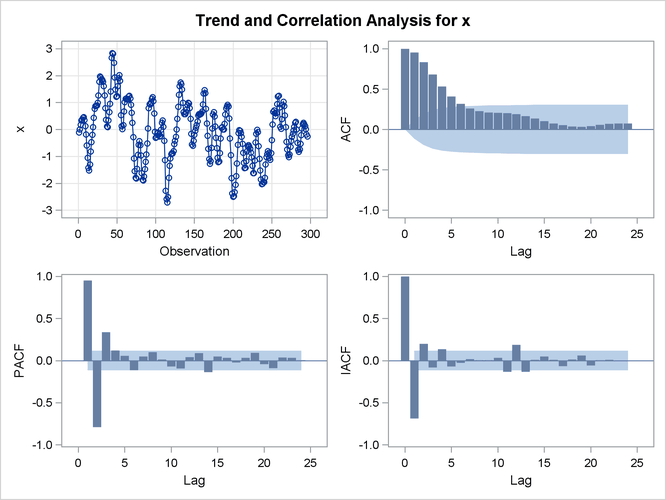
The ESTIMATE statement results for the AR(3) model for the input series X are shown in Output 7.3.3.
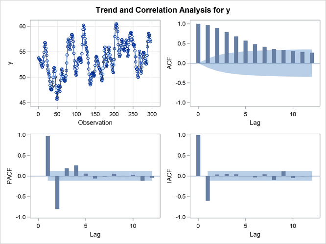
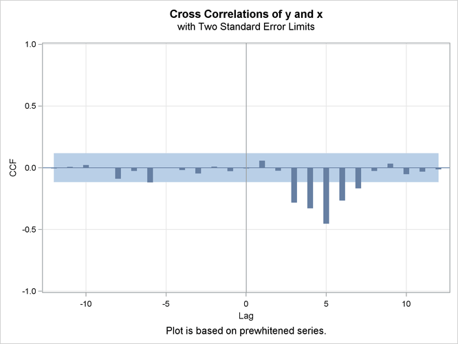
The IDENTIFY statement results for the dependent series Y cross-correlated with the input series X are shown in Output 7.3.4, Output 7.3.5, Output 7.3.6, and Output 7.3.7. Since a model has been fit to X, both Y and X are prewhitened by this model before the sample cross-correlations are computed.
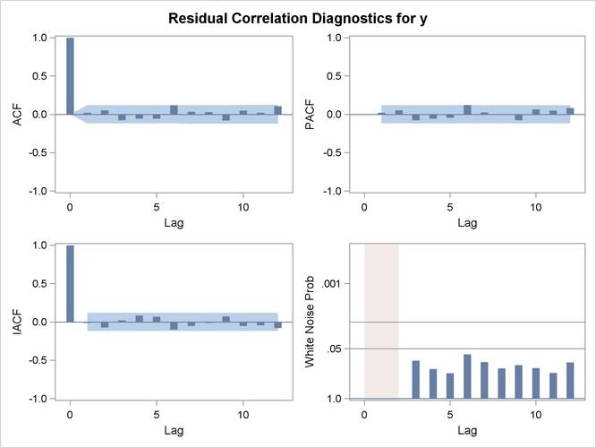
The ESTIMATE statement results for the transfer function model with no structure on the noise term are shown in Output 7.3.8, Output 7.3.9, and Output 7.3.10.
Output 7.3.8: Estimation Output of the First Transfer Function Model
| Conditional Least Squares Estimation | |||||||
|---|---|---|---|---|---|---|---|
| Parameter | Estimate | Standard Error |
t Value | Approx Pr > |t| |
Lag | Variable | Shift |
| MU | 53.32256 | 0.04926 | 1082.51 | <.0001 | 0 | y | 0 |
| NUM1 | -0.56467 | 0.22405 | -2.52 | 0.0123 | 0 | x | 3 |
| NUM1,1 | 0.42623 | 0.46472 | 0.92 | 0.3598 | 1 | x | 3 |
| NUM1,2 | 0.29914 | 0.35506 | 0.84 | 0.4002 | 2 | x | 3 |
| DEN1,1 | 0.60073 | 0.04101 | 14.65 | <.0001 | 1 | x | 3 |
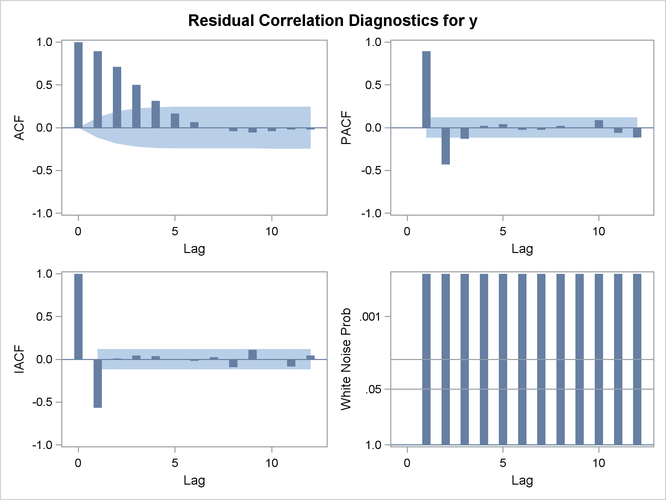
The residual correlation analysis suggests an AR(2) model for the noise part of the model. The ESTIMATE statement results for the final transfer function model with AR(2) noise are shown in Output 7.3.11.
Output 7.3.11: Estimation Output of the Final Model
| Conditional Least Squares Estimation | |||||||
|---|---|---|---|---|---|---|---|
| Parameter | Estimate | Standard Error |
t Value | Approx Pr > |t| |
Lag | Variable | Shift |
| MU | 53.26304 | 0.11929 | 446.48 | <.0001 | 0 | y | 0 |
| AR1,1 | 1.53291 | 0.04754 | 32.25 | <.0001 | 1 | y | 0 |
| AR1,2 | -0.63297 | 0.05006 | -12.64 | <.0001 | 2 | y | 0 |
| NUM1 | -0.53522 | 0.07482 | -7.15 | <.0001 | 0 | x | 3 |
| NUM1,1 | 0.37603 | 0.10287 | 3.66 | 0.0003 | 1 | x | 3 |
| NUM1,2 | 0.51895 | 0.10783 | 4.81 | <.0001 | 2 | x | 3 |
| DEN1,1 | 0.54841 | 0.03822 | 14.35 | <.0001 | 1 | x | 3 |