The GLIMMIX Procedure
-
Overview

-
Getting Started
-
SyntaxPROC GLIMMIX StatementBY StatementCLASS StatementCODE StatementCONTRAST StatementCOVTEST StatementEFFECT StatementESTIMATE StatementFREQ StatementID StatementLSMEANS StatementLSMESTIMATE StatementMODEL StatementNLOPTIONS StatementOUTPUT StatementPARMS StatementRANDOM StatementSLICE StatementSTORE StatementWEIGHT StatementProgramming StatementsUser-Defined Link or Variance Function
-
DetailsGeneralized Linear Models TheoryGeneralized Linear Mixed Models TheoryGLM Mode or GLMM ModeStatistical Inference for Covariance ParametersDegrees of Freedom MethodsEmpirical Covariance ("Sandwich") EstimatorsExploring and Comparing Covariance MatricesProcessing by SubjectsRadial Smoothing Based on Mixed ModelsOdds and Odds Ratio EstimationParameterization of Generalized Linear Mixed ModelsResponse-Level Ordering and ReferencingComparing the GLIMMIX and MIXED ProceduresSingly or Doubly Iterative FittingDefault Estimation TechniquesDefault OutputNotes on Output StatisticsODS Table NamesODS Graphics
-
ExamplesBinomial Counts in Randomized BlocksMating Experiment with Crossed Random EffectsSmoothing Disease Rates; Standardized Mortality RatiosQuasi-likelihood Estimation for Proportions with Unknown DistributionJoint Modeling of Binary and Count DataRadial Smoothing of Repeated Measures DataIsotonic Contrasts for Ordered AlternativesAdjusted Covariance Matrices of Fixed EffectsTesting Equality of Covariance and Correlation MatricesMultiple Trends Correspond to Multiple Extrema in Profile LikelihoodsMaximum Likelihood in Proportional Odds Model with Random EffectsFitting a Marginal (GEE-Type) ModelResponse Surface Comparisons with Multiplicity AdjustmentsGeneralized Poisson Mixed Model for Overdispersed Count DataComparing Multiple B-SplinesDiallel Experiment with Multimember Random EffectsLinear Inference Based on Summary DataWeighted Multilevel Model for Survey DataQuadrature Method for Multilevel Model
- References
The Odds Ratio Estimates Table
This table is produced by the ODDSRATIO option in the MODEL statement. It consists of estimates of odds ratios and their confidence limits. Odds ratios are produced for the following:
-
classification main effects, if they appear in the MODEL statement
-
continuous variables in the MODEL statement, unless they appear in an interaction with a classification effect
-
continuous variables in the MODEL statement at fixed levels of a classification effect, if the MODEL statement contains an interaction of the two.
-
continuous variables in the MODEL statements if they interact with other continuous variables
The Default Table
Consider the following PROC GLIMMIX statements that fit a logistic model with one classification effect, one continuous variable, and their interaction (the ODDSRATIO option in the MODEL statement requests the "Odds Ratio Estimates" table).
proc glimmix;
   class A;
   model y = A x A*x / dist=binary oddsratio;
run;
By default, odds ratios are computed as follows:
-
The covariate is set to its average,
 , and the least squares means for the A effect are obtained. Suppose
  denotes the matrix of coefficients defining the estimable functions that produce the a least squares means
  , and
, and  denotes the jth row of . Differences of the least squares means against the last level of the
 Afactor are computed and exponentiated: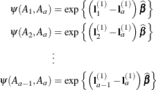
The differences are checked for estimability. Notice that this set of odds ratios can also be obtained with the following LSMESTIMATE statement (assuming
Ahas five levels):lsmestimate A 1 0 0 0 -1, 0 1 0 0 -1, 0 0 1 0 -1, 0 0 0 1 -1 / exp cl;You can also obtain the odds ratios with this LSMEANS statement (assuming the last level of
Ais coded as 5):lsmeans A / diff=control('5') oddsratio cl; -
The odds ratios for the covariate must take into account that
xoccurs in an interaction with theAeffect. A second set of least squares means are computed, wherexis set to . Denote the coefficients of the estimable functions for this set of least squares means as
  . Differences of the least squares means at a given level of factor
 Aare then computed and exponentiated: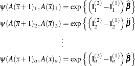
The differences are checked for estimability. If the continuous covariate does not appear in an interaction with the
Avariable, only a single odds ratio estimate related toxwould be produced, relating the odds of a one-unit shift in the regressor from.
Suppose you fit a model that contains interactions of continuous variables, as with the following statements:
proc glimmix;
   class A;
   model y = A x x*z / dist=binary oddsratio;
run;
In the computation of the A least squares means, the continuous effects are set to their means—that is, and  . In the computation of odds ratios for
 x, linear predictors are computed at x = , x*z =  and at
 x = , x*z =  .
.
Modifying the Default Table, Customized Odds Ratios
Several suboptions of the ODDSRATIO option in the MODEL statement are available to obtain customized odds ratio estimates. For customized odds ratios that cannot be obtained with these suboptions, use the EXP option in the ESTIMATE or LSMESTIMATE statement.
The type of differences constructed when the levels of a classification factor are varied is controlled by the DIFF= suboption. By default, differences against the last level are taken. DIFF=FIRST computes differences from the first level, and DIFF=ALL computes odds ratios based on all pairwise differences.
For continuous variables in the model, you can change both the reference value (with the AT suboption) and the units of change
(with the UNIT suboption). By default, a one-unit change from the mean of the covariate is assessed. For example, the following
statements produce all pairwise differences for the A factor:
proc glimmix;
   class A;
   model y = A x A*x / dist=binary
                       oddsratio(diff=all
                                 at   x=4
                                 unit x=3);
run;
The covariate x is set to the reference value x = 4 in the computation of the least squares means for the A odds ratio estimates. The odds ratios computed for the covariate are based on differencing this set of least squares means
with a set of least squares means computed at  .
.