The OPTGRAPH Procedure

Example 1.3 Betweenness and Closeness Centrality for Computer Network Topology

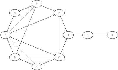
Consider a small network of 10 computers spread out across an office. Let a node represent a computer, and let a link represent a direct connection between the machines. For this example, consider the links as Ethernet connections that enable data to transfer between computers. If two computers are not connected directly, then the information must flow through other connected machines. Consider a topology as shown in Figure 1.142. This is an example of the well-known kite network, which was popularized by David Krackhardt (1990) for better understanding of social networks in the workplace.

Figure 1.142: Office Computer Network

Define the link data set as follows:

data LinkSetInCompNet;
   input from $ to $ @@;
   datalines;
A B  A C  A D  B C  B D
B E  C D  C F  C H  D E
D F  D G  E F  E G  F G
F H  H I  I J
;

To better understand the topology of the computer network, calculate the degree, closeness, and betweenness centrality. It is also interesting to look for articulation points in the computer network to identify places of vulnerability. All of these calculations can be done in one call to PROC OPTGRAPH as follows:

proc optgraph
   data_links = LinkSetInCompNet
   out_links  = LinkSetOut
   out_nodes  = NodeSetOut;
   centrality
      degree  = out
      close   = unweight
      between = unweight;
   biconcomp;
run;

Output 1.3.1 shows the resulting node data set NodeSetOut sorted by closeness.

Output 1.3.1: Node Closeness and Betweenness Centrality, Sorted by Closeness

node	centr_degree_out	centr_close_unwt	centr_between_unwt	artpoint
C	5	0.64286	0.23148	0
F	5	0.64286	0.23148	0
D	6	0.60000	0.10185	0
H	3	0.60000	0.38889	1
B	4	0.52941	0.02315	0
E	4	0.52941	0.02315	0
A	3	0.50000	0.00000	0
G	3	0.50000	0.00000	0
I	2	0.42857	0.22222	1
J	1	0.31034	0.00000	0

Output 1.3.2 shows the resulting node (NodeSetOut) and link data sets (LinkSetOut) sorted by betweenness.

Output 1.3.2: Node Closeness and Betweenness Centrality, Sorted by Betweenness

Obs	node	centr_degree_out	centr_close_unwt	centr_between_unwt	artpoint
1	H	3	0.60000	0.38889	1
2	C	5	0.64286	0.23148	0
3	F	5	0.64286	0.23148	0
4	I	2	0.42857	0.22222	1
5	D	6	0.60000	0.10185	0
6	E	4	0.52941	0.02315	0
7	B	4	0.52941	0.02315	0
8	A	3	0.50000	0.00000	0
9	G	3	0.50000	0.00000	0
10	J	1	0.31034	0.00000	0

Obs	from	to	biconcomp	centr_between_unwt
1	H	I	2	0.44444
2	C	H	3	0.29167
3	F	H	3	0.29167
4	I	J	1	0.25000
5	E	F	3	0.12963
6	B	C	3	0.12963
7	A	C	3	0.12500
8	F	G	3	0.12500
9	C	D	3	0.09259
10	D	F	3	0.09259
11	A	D	3	0.08333
12	D	G	3	0.08333
13	C	F	3	0.07407
14	B	E	3	0.07407
15	B	D	3	0.05093
16	D	E	3	0.05093
17	A	B	3	0.04167
18	E	G	3	0.04167

The computers with the highest closeness centrality are C and F, because they have the shortest paths to all other nodes. These computers are key to the efficient distribution of information across the network. Assuming that the entire office has some centralized data that should be shared with all computers, machines C and F would be the best candidates for storing the data on their local hard drives. The computer with the highest betweenness centrality is H. Although machine H has only three connections, it is one of the most important machines in the office because it serves as the only way to reach computers I and J from the other machines in the office. Notice also that machine H is an articulation point because removing it would disconnect the office network. In this setting, computers with high betweenness should be carefully maintained and secured with UPS (uninterruptible power supply) systems to ensure they are always online.