The OPTGRAPH Procedure
- Overview
-
Getting Started

-
SyntaxFunctional SummaryPROC OPTGRAPH StatementBICONCOMP StatementCENTRALITY StatementCLIQUE StatementCOMMUNITY StatementCONCOMP StatementCORE StatementCYCLE StatementDATA_LINKS_VAR StatementDATA_MATRIX_VAR StatementDATA_NODES_VAR StatementEIGENVECTOR StatementLINEAR_ASSIGNMENT StatementMINCOSTFLOW StatementMINCUT StatementMINSPANTREE StatementPERFORMANCE StatementREACH StatementSHORTPATH StatementSUMMARY StatementTRANSITIVE_CLOSURE StatementTSP Statement
-
DetailsGraph Input DataMatrix Input DataData Input OrderParallel ProcessingNumeric LimitationsSize LimitationsCommon Notation and AssumptionsBiconnected Components and Articulation PointsCentralityCliqueCommunityConnected ComponentsCore DecompositionCycleEigenvector ProblemLinear Assignment (Matching)Minimum-Cost Network FlowMinimum CutMinimum Spanning TreeReach (Ego) NetworkShortest PathSummaryTransitive ClosureTraveling Salesman ProblemMacro VariablesODS Table Names
-
ExamplesArticulation Points in a Terrorist NetworkInfluence Centrality for Project Groups in a Research DepartmentBetweenness and Closeness Centrality for Computer Network TopologyBetweenness and Closeness Centrality for Project Groups in a Research DepartmentEigenvector Centrality for Word Sense DisambiguationCentrality Metrics for Project Groups in a Research DepartmentCommunity Detection on Zachary’s Karate Club DataRecursive Community Detection on Zachary’s Karate Club DataCycle Detection for Kidney Donor ExchangeLinear Assignment Problem for Minimizing Swim TimesLinear Assignment Problem, Sparse Format versus Dense FormatMinimum Spanning Tree for Computer Network TopologyTransitive Closure for Identification of Circular Dependencies in a Bug Tracking SystemReach Networks for Computation of Market Coverage of a Terrorist NetworkTraveling Salesman Tour through US Capital Cities
- References
Centrality
In general terms, the centrality of a node or link in a graph gives some indication of its relative importance within a graph. In the field of network analysis, many different types of centrality metrics are used to better understand levels of prominence. For a good review of centrality metrics, see Newman 2010.
You can use the CENTRALITY statement in PROC OPTGRAPH to calculate several of these metrics. The options for this statement are described in the section CENTRALITY Statement.
The CENTRALITY statement reports status information in a macro variable called _OPTGRAPH_CENTRALITY_. See the section Macro Variable _OPTGRAPH_CENTRALITY_ for more information about this macro variable.
The following sections describe each of the possible centrality metrics that can be calculated in PROC OPTGRAPH.
Degree Centrality
The degree of a node v in an undirected graph is the number of links that are incident to node v. The out-degree of a node in a directed graph is the number of out-links incident to that node; the in-degree is the number of in-links incident. The term degree and out-degree are interchangeable for an undirected graph. Degree centrality is simply the (in- or out-) degree of a node and can be interpreted as some form of relative importance to a network. For example, in a network where nodes are people and you are tracking the flow of a virus, the degree centrality gives some idea of the magnitude of the risk of spreading the virus. People with a higher out-degree can lead to a quicker and more widespread transmission. In a friendship network, in-degree often indicates popularity.
Degree centrality is calculated according to the value specified for the DEGREE= option in the CENTRALITY statement. The results are provided in the node output data set that is specified in the OUT_NODES= option in the PROC OPTGRAPH statement.
The algorithm used by PROC OPTGRAPH to compute degree centrality is a simple lookup, runs in time ![]() , and therefore should scale to very large graphs.
, and therefore should scale to very large graphs.
As a simple example, consider again the directed graph in Figure 1.8 with data set LinkSetIn defined in the section Link Input Data. The following statements calculate the degree centrality for both in- and out-degree:
proc optgraph
   graph_direction = directed
   data_links      = LinkSetIn
   out_nodes       = NodeSetOut;
   centrality
      degree       = both;
run;
The node data set NodeSetOut now contains the degree centrality of the input graph. For a directed graph, the data set provides the in-degree (variable
centr_degree_in), the out-degree (variable centr_degree_out), and the degree that is the sum of in- and out-degrees (variable centr_degree). This data set is shown in Figure 1.22.
Figure 1.22: Degree Centrality of a Simple Directed Graph
Influence Centrality
Influence centrality is a generalization of degree centrality that considers the link and node weights of adjacent nodes (![]() ) in addition to the link weights of nodes that are adjacent to adjacent nodes (
) in addition to the link weights of nodes that are adjacent to adjacent nodes (![]() ). The metric
). The metric ![]() is referred to as first-order influence centrality, and the metric
is referred to as first-order influence centrality, and the metric ![]() is referred to as second-order influence centrality.
is referred to as second-order influence centrality.
Let ![]() define the link weight for link
define the link weight for link ![]() , and let
, and let ![]() define the node weight for node u. Let
define the node weight for node u. Let ![]() represent the list of nodes connected to node u (that is, its neighbors); this list is called the adjacency list. For directed graphs, the neighbors are the out-links. The
general formula for influence centrality is
represent the list of nodes connected to node u (that is, its neighbors); this list is called the adjacency list. For directed graphs, the neighbors are the out-links. The
general formula for influence centrality is
![\begin{eqnarray*} C_1(u) & = & \frac{ \sum _{v \in \delta _ u} w_{uv} }{ \sum _{v \in N } w_ v }\\[0.1in] C_2(u) & = & \sum _{v \in \delta _ u} C_1(v) \end{eqnarray*}](images/procgralg_optgraph0040.png)
As the name suggests, this metric gives some indication of potential influence, performance, or ability to transfer knowledge.
Influence centrality is calculated according to the value of the INFLUENCE= option in the CENTRALITY statement. The results are provided in the node output data set that is specified in the OUT_NODES= option in the PROC OPTGRAPH statement.
The algorithm used by PROC OPTGRAPH to compute influence centrality is a simple traversal, runs in time ![]() , and therefore should scale to very large graphs.
, and therefore should scale to very large graphs.
Consider again the directed graph in Figure 1.8. Ignore the weights and just calculate the ![]() and
and ![]() metrics based on connections (that is, consider all link and node weights as 1). The following statements calculate the unweighted
influence centrality:
metrics based on connections (that is, consider all link and node weights as 1). The following statements calculate the unweighted
influence centrality:
proc optgraph
   graph_direction = directed
   data_links      = LinkSetIn
   out_nodes       = NodeSetOut;
   centrality
      influence    = unweight;
run;
The node data set NodeSetOut now contains the unweighted influence centrality of the input graph, including the ![]() variable
variable centr_influence1_unwt and the ![]() variable
variable centr_influence2_unwt. This data set is shown in Figure 1.23.
Figure 1.23: Influence Centrality of a Simple Directed Graph
For a more detailed example, see Influence Centrality for Project Groups in a Research Department.
Clustering Coefficient
The clustering coefficient for a node is the number of links between the nodes within its neighborhood divided by the number of links that could possibly exist between them (their induced complete graph).
Let ![]() represent the list of nodes that are connected to node u (excluding itself). The formula for the clustering coefficient is:
represent the list of nodes that are connected to node u (excluding itself). The formula for the clustering coefficient is:
For a particular node i, the clustering coefficient determines how close to being a clique (complete subgraph) the subgraph induced its neighbor
set ![]() are. In social networks, a high clustering coefficient can help predict relationships that might not be known, confirmed,
or realized yet. The fact that person i knows person j and person j knows person k does not guarantee that person i knows person k, but it is much more likely that person i knows person k than that person i knows some random person.
are. In social networks, a high clustering coefficient can help predict relationships that might not be known, confirmed,
or realized yet. The fact that person i knows person j and person j knows person k does not guarantee that person i knows person k, but it is much more likely that person i knows person k than that person i knows some random person.
The clustering coefficient is calculated when the CLUSTERING_COEF option is specified in the CENTRALITY statement. The results are provided in the node output data set that is specified in the OUT_NODES= option in the PROC OPTGRAPH statement.
The algorithm used by PROC OPTGRAPH to compute the clustering coefficient is a relatively simple traversal, runs in time ![]() , and therefore should scale to very large graphs.
, and therefore should scale to very large graphs.
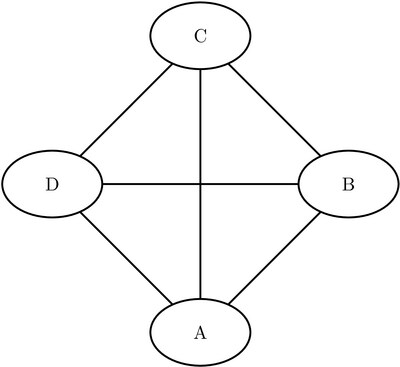
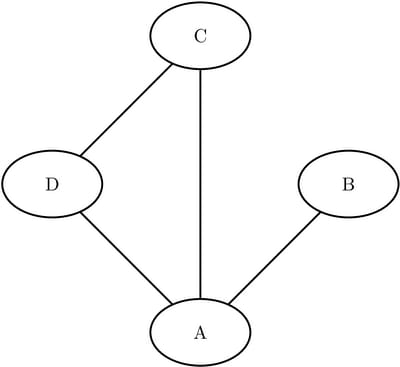
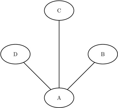
Consider the three undirected graphs on four nodes shown in Figure Figure 1.24.
Figure 1.24: Three Undirected Graphs
|
Graph 1 |
Graph 2 |
Graph 3 |
|
|
||
|
|
|
|
Define the three link data sets as follows:
data LinkSetInCC1;
   input from $ to $ @@;
   datalines;
A B  A C  A D
B C  B D  C D
;

data LinkSetInCC2;
   input from $ to $ @@;
   datalines;
A B  A C  A D
C D
;

data LinkSetInCC3;
   input from $ to $ @@;
   datalines;
A B  A C  A D
;
The following statements use three calls to PROC OPTGRAPH to calculate the clustering coefficients for each graph:
proc optgraph
   data_links = LinkSetInCC1
   out_nodes  = NodeSetOut1;
   centrality
      clustering_coef;
run;

proc optgraph
   data_links = LinkSetInCC2
   out_nodes  = NodeSetOut2;
   centrality
      clustering_coef;
run;

proc optgraph
   data_links = LinkSetInCC3
   out_nodes  = NodeSetOut3;
   centrality
      clustering_coef;
run;
The node data sets provide the clustering coefficients for each graph (variable centr_cluster) as shown in Figure 1.25 through Figure 1.27.
Figure 1.25: Clustering Coefficient of a Simple Undirected Graph 1
Figure 1.26: Clustering Coefficient of a Simple Undirected Graph 2
Figure 1.27: Clustering Coefficient of a Simple Undirected Graph 3
Closeness Centrality
Closeness centrality is the reciprocal of the average of the shortest path (geodesic) distances from a particular node to all other nodes. Closeness can be thought of as a measure of how long it takes information to spread from a particular node to other nodes in the network.
Define ![]() to be the shortest path distance from node u to node v.
to be the shortest path distance from node u to node v.
Closeness Centrality for an Undirected Graph
For an undirected graph, ![]() is the set of reachable nodes from node u. The set of unreachable nodes from node u is
is the set of reachable nodes from node u. The set of unreachable nodes from node u is ![]() . The CLOSE_NOPATH=
option specifies how to handle unreachable nodes.
. The CLOSE_NOPATH=
option specifies how to handle unreachable nodes.
For the special case in which all nodes are unreachable from node u, the closeness centrality is defined as 0. Otherwise, closeness centrality is calculated as
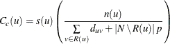
where p defines a penalty parameter for unreachable nodes, ![]() defines the number of nodes that are considered in calculating the average, and
defines the number of nodes that are considered in calculating the average, and ![]() is a scaling factor, as shown in Table 1.56.
is a scaling factor, as shown in Table 1.56.
Table 1.56: Formulas for CLOSE_NOPATH= Option for Undirected Graphs
|
CLOSE_NOPATH= |
p |
|
|
|
DIAMETER |
|
|
1 |
|
NNODES |
|
|
1 |
|
ZERO |
0 |
|
|
Closeness Centrality for a Directed Graph
For a directed graph, ![]() is the set of reachable nodes from node u, whereas
is the set of reachable nodes from node u, whereas ![]() is the set of nodes from which a finite path exists to node u. The set of unreachable nodes from node u is
is the set of nodes from which a finite path exists to node u. The set of unreachable nodes from node u is ![]() , whereas the set of nodes from which a finite path to node u does not exist is
, whereas the set of nodes from which a finite path to node u does not exist is ![]() .
.
For the special case in which all nodes are unreachable from node u, the out-closeness centrality is defined as 0. Otherwise, out-closeness centrality is calculated as
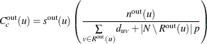
where ![]() defines the number of nodes that are considered in calculating the average and
defines the number of nodes that are considered in calculating the average and ![]() is a scaling factor, as shown in Table 1.57:
is a scaling factor, as shown in Table 1.57:
For the special case in which node u is unreachable from all other nodes, the in-closeness centrality is defined as 0. Otherwise, in-closeness centrality is calculated as
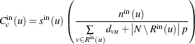
where ![]() defines the number of nodes that are considered in calculating the average and
defines the number of nodes that are considered in calculating the average and ![]() is a scaling factor, as shown in Table 1.57.
is a scaling factor, as shown in Table 1.57.
Table 1.57: Formulas for CLOSE_NOPATH= Option for Directed Graphs
|
CLOSE_NOPATH= |
|
|
|
|
|
DIAMETER |
|
1 |
|
1 |
|
NNODES |
|
1 |
|
1 |
|
ZERO |
|
|
|
|
The overall closeness centrality for directed graphs is calculated as
Harmonic Centrality
Harmonic centrality, as described in Rochat (2009), is a variant of closeness centrality that attempts to simplify the treatment of unreachable nodes by calculating the average of the reciprocal of the shortest path distances from a particular node to all other nodes. The formula for harmonic centrality is:
To enable the calculation of harmonic centrality, use the CLOSE_NOPATH=HARMONIC option.
Closeness centrality is calculated according to the value of the CLOSE= option in the CENTRALITY statement. The results are provided in the node output data set that is specified in the OUT_NODES= option in the PROC OPTGRAPH statement. If CLOSE=WEIGHT (or BOTH), then the shortest paths are calculated with respect to the weighted graph. Because the metric uses shortest paths to determine closeness, the weight and the closeness metric are inversely related. In general, the lower the weight, the higher the contribution to the closeness metric.
The algorithm that PROC OPTGRAPH uses to compute closeness centrality relies on calculating shortest paths for all source-sink
pairs and runs in time ![]() . Therefore, this algorithm is not expected to scale to very large graphs. Because the shortest path computations can be calculated
independently (for each source node), you can speed up the algorithm by specifying the NTHREADS= option in the PERFORMANCE
statement.
. Therefore, this algorithm is not expected to scale to very large graphs. Because the shortest path computations can be calculated
independently (for each source node), you can speed up the algorithm by specifying the NTHREADS= option in the PERFORMANCE
statement.
Consider again the directed graph in Figure 1.8 with the data set LinkSetIn, which is defined in the section Link Input Data. The following statements calculate the closeness centrality for both the weighted and unweighted graphs:
proc optgraph
   graph_direction = directed
   data_links      = LinkSetIn
   out_nodes       = NodeSetOut;
   centrality
      close        = both;
run;
The node data set NodeSetOut now contains the weighted and unweighted directed closeness centrality of the input graph. The data set provides the unweighted
closeness (the centr_close_unwt variable), in-closeness (the centr_close_in_unwt variable), and out-closeness (the centr_close_out_unwt variable). It also provides the weighted variants centr_close_wt, centr_close_in_wt, and centr_close_out_wt. This data set is shown in Figure 1.28.
Figure 1.28: Closeness Centrality of a Simple Directed Graph
| node | centr_close_wt | centr_close_in_wt | centr_close_out_wt | centr_close_unwt | centr_close_in_unwt | centr_close_out_unwt |
|---|---|---|---|---|---|---|
| 0 | 0.31250 | 0.25000 | 0.37500 | 0.38095 | 0.33333 | 0.42857 |
| 1 | 0.30303 | 0.33333 | 0.27273 | 0.38095 | 0.42857 | 0.33333 |
| 3 | 0.16667 | 0.00000 | 0.33333 | 0.25000 | 0.00000 | 0.50000 |
| 5 | 0.21429 | 0.42857 | 0.00000 | 0.25000 | 0.50000 | 0.00000 |
Betweenness Centrality
Betweenness centrality counts the number of times a particular node (or link) occurs on shortest paths between other nodes. Betweenness can be thought of as a measure of the control that a node (or link) has over the communication flow among the rest of the network. In this sense, the nodes (or links) that have high betweenness are the gatekeepers of information, because of their relative location in the network.
The formula for node betweenness centrality is
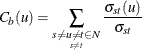
where ![]() is the number of shortest paths from s to t and
is the number of shortest paths from s to t and ![]() is the number of shortest paths from s to t that pass through node u.
is the number of shortest paths from s to t that pass through node u.
The formula for link betweenness centrality is
where ![]() is the number of shortest paths from s to t that pass through link
is the number of shortest paths from s to t that pass through link ![]() .
.
By default, this metric is normalized by dividing through by two times the number of pairs of nodes, not including u, which is ![]() . You can disable this normalization by using the BETWEEN_NORM=
option.
. You can disable this normalization by using the BETWEEN_NORM=
option.
For directed graphs, because the paths are directed, only the out-betweenness is computed. To get the in-betweenness, you must reverse all the directions of the graph and run the procedure again. This can be accomplished by simply using the DATA_LINKS_VAR statement to reverse the interpretation of from and to.
Betweenness centrality is calculated according to the value of the BETWEEN= option in the CENTRALITY statement. The node betweenness results are provided in the node output data set that is specified in the OUT_NODES= option in the PROC OPTGRAPH statement. The link betweenness results are provided in the link output data set that is specified in the OUT_LINKS= option in the PROC OPTGRAPH statement. Like closeness, if BETWEEN=WEIGHT (or BOTH), then the calculation of shortest paths is done using the weighted graph. Because the metric uses shortest paths to determine betweenness, the weight and the betweenness metric are inversely related. In general the lower the weight, the higher the contribution to the betweenness metric.
The algorithm used by PROC OPTGRAPH to compute betweenness centrality relies on calculating shortest paths for all source-sink
pairs and runs in time ![]() . Therefore, it is not expected to scale to very large graphs. Similar to closeness centrality, because shortest path computations
can be calculated independently (for each source node), the algorithm can be sped up by using the NTHREADS= option in the
PERFORMANCE
statement. When closeness and betweenness centrality are run together, PROC OPTGRAPH calculates both metrics in one run.
. Therefore, it is not expected to scale to very large graphs. Similar to closeness centrality, because shortest path computations
can be calculated independently (for each source node), the algorithm can be sped up by using the NTHREADS= option in the
PERFORMANCE
statement. When closeness and betweenness centrality are run together, PROC OPTGRAPH calculates both metrics in one run.
Consider again the directed graph in Figure 1.8 with data set LinkSetIn defined in the section Link Input Data. The following statements calculate the betweenness centrality for both the weighted and unweighted graphs:
proc optgraph
   graph_direction = directed
   data_links      = LinkSetIn
   out_links       = LinkSetOut
   out_nodes       = NodeSetOut;
   centrality
      between      = both;
run;
The node data set NodeSetOut now contains the weighted (variable centr_between_wt) and unweighted (variable centr_between_unwt) node betweenness centrality of the input graph. This data set is shown in Figure 1.29.
Figure 1.29: Node Betweenness Centrality of a Simple Directed Graph
In addition, the link data set LinkSetOut contains the weighted (variable centr_between_wt) and unweighted (variable centr_between_unwt) link betweenness centrality of the input graph. This data set is shown in Figure 1.30.
Figure 1.30: Link Betweenness Centrality of a Simple Directed Graph
For more detailed examples, see Betweenness and Closeness Centrality for Computer Network Topology and Betweenness and Closeness Centrality for Project Groups in a Research Department.
Eigenvector Centrality
Eigenvector centrality is an extension of degree centrality in which centrality points are awarded for each neighbor. However, not all neighbors are equally important. Intuitively, a connection to an important node should contribute more to the centrality score than a connection to a less important node. This is the basic idea behind eigenvector centrality. Eigenvector centrality of a node is defined to be proportional to the sum of the scores of all nodes that are connected to it. Mathematically, it is
where ![]() is the eigenvector centrality of node i,
is the eigenvector centrality of node i, ![]() is a constant,
is a constant, ![]() is the set of nodes that connect to node i, and
is the set of nodes that connect to node i, and ![]() is the weight of the link from node i to node j.
is the weight of the link from node i to node j.
Eigenvector centrality can be written as an eigenvector equation in matrix form as
As the preceding equation shows, x is the eigenvector and ![]() is the eigenvalue. Because x should be positive, only the principal eigenvector that corresponds to the largest eigenvalue is of interest.
is the eigenvalue. Because x should be positive, only the principal eigenvector that corresponds to the largest eigenvalue is of interest.
Eigenvector centrality is calculated according to the value that you specify in the EIGEN= option in the CENTRALITY statement. The results are provided in the node output data set that you specify in the OUT_NODES= option in the PROC OPTGRAPH statement.
The following example illustrates the use of eigenvector centrality on the undirected graph G shown in Figure 1.31.
Figure 1.31: Eigenvector Centrality Example of a Simple Undirected Graph
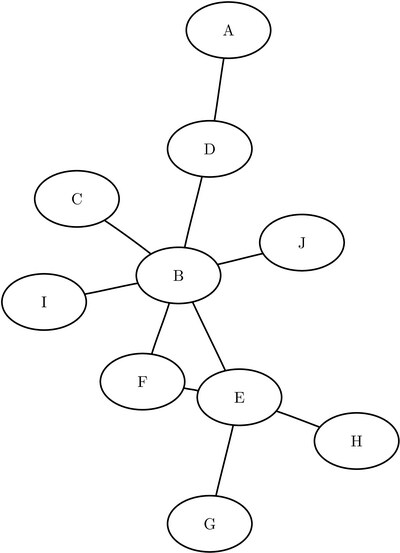
The graph can be represented by the following links data set LinkSetIn:
data LinkSetIn;
   input from $ to $ @@;
   datalines;
A D  B C  B D  B E  B F
B I  B J  E F  E G  E H
;
The following statements compute the eigenvector centrality:
proc optgraph
   data_links        = LinkSetIn
   out_nodes         = NodeSetOut;
   centrality
      eigen          = unweight;
run;
The data set NodeSetOut now contains the eigenvector centrality of each node. It is shown in Figure 1.32.
Figure 1.32: Eigenvector Centrality Output
Even though nodes F and D both have the same degree of 2, node F has a higher eigenvector centrality than node D. This is because node F links to two important nodes (B and E), whereas node D links to one important node (B) and one unimportant node (A).
For a more detailed example, see Eigenvector Centrality for Word Sense Disambiguation.
Hub and Authority Scoring
Hub and authority centrality was originally developed by Kleinberg (1998) to rank the importance of web pages. Certain web pages are important in the sense that they point to many important pages (called hubs). On the other hand, some web pages are important because they are pointed to by many important pages (called authorities). In other words, a good hub node is one that points to many good authorities, and a good authority node is one that is pointed to by many good hub nodes. This idea can be applied to many other types of graphs besides web pages. For example, it can be applied to a citation network for journal articles. A review article that cites many good authority papers has a high hub score, whereas a paper that is referenced by many other papers has a high authority score. The section Authority in U.S. Supreme Court Precedence shows a similar example.
The authority centrality of a node is proportional to the sum of the hub centrality of nodes that point to it. Similarly, the hub centrality of a node is proportional to the sum of the authorities of nodes that it points to. That is,
where ![]() is the authority centrality of node i,
is the authority centrality of node i, ![]() is the hub centrality of node i,
is the hub centrality of node i, ![]() is the weight of the link from node i to node j, and
is the weight of the link from node i to node j, and ![]() and
and ![]() are constants.
are constants.
The definition can be written in matrix form as follows:
Thus, the authority and hub centralities are the principal eigenvectors of ![]() and
and ![]() , respectively. To solve this eigenvector problem, PROC OPTGRAPH provides two algorithms: the Jacobi-Davidson algorithm and
the power method. You use the EIGEN_ALGORITHM= option in the CENTRALITY statement to specify which algorithm to use. JACOBI_DAVIDSON,
which is the default, is a state-of-the-art package for solving large-scale eigenvalue problems (Sleijpen and van der Vorst
2000). The power method is one of the standard algorithms for solving eigenvalue problems, but it converges slowly for certain
problems.
, respectively. To solve this eigenvector problem, PROC OPTGRAPH provides two algorithms: the Jacobi-Davidson algorithm and
the power method. You use the EIGEN_ALGORITHM= option in the CENTRALITY statement to specify which algorithm to use. JACOBI_DAVIDSON,
which is the default, is a state-of-the-art package for solving large-scale eigenvalue problems (Sleijpen and van der Vorst
2000). The power method is one of the standard algorithms for solving eigenvalue problems, but it converges slowly for certain
problems.
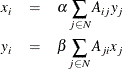
The following example illustrates the use of hub and authority scoring on the directed graph G shown in Figure 1.33. Each node represents a web page. If web page i has a hyperlink that points to web page j, then there is a directed link from i to j.
Figure 1.33: Hub and Authority Centrality Example of a Simple Directed Graph
The graph can be represented by the following links data set LinkSetIn:
data LinkSetIn;
   input from $ to $ @@;
   datalines;
B C  C B  D A  D B  E B
E D  E F  F B  F E  G E
H E  I E  I B  J E  J B
K B  K E
;
The following statements compute hub and authority centrality:
proc optgraph
   graph_direction   = directed
   data_links        = LinkSetIn
   out_nodes         = NodeSetOut;
   centrality
      hub            = unweight
      auth           = unweight;
run;
The data set NodeSetOut now contains the hub and authority scores of each node. It is shown in Figure 1.34.
Figure 1.34: Hub and Authority Centrality Output
The output shows that nodes B and E have high authority scores because they have many incoming links. Nodes F, I, J, K have high hub scores because they all point to good authority nodes B and E.
Weight Interpretation
In certain situations, you might want to calculate various centrality metrics on the same weighted graph. As described above, closeness and betweenness centrality have inverse relationships with the link weights, because these metrics are calculated using shortest paths. So the lower the weight, the higher the contribution to the centrality metric. All of the other metrics are direct relationships. That is, the higher the weight, the higher the contribution to the centrality metric.
To calculate these metrics in one invocation of PROC OPTGRAPH, you can use the WEIGHT2= option. The variable defined by this option is used as link weights for closeness and betweenness calculations whereas all other metrics use the standard weight variable.
For a more detailed example, see Centrality Metrics for Project Groups in a Research Department, which uses the WEIGHT2= option.
Processing by Cluster
You can process a number of induced subgraphs of a graph with only one call to PROC OPTGRAPH by using the BY_CLUSTER option in the CENTRALITY statement. This section shows an example of how to use this option.
Centrality by Cluster for a Simple Undirected Graph
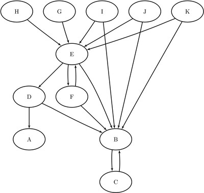
Consider the graph depicted in Figure 1.35.
Figure 1.35: Undirected Graph
The following statements create the data set LinkSetIn:
data LinkSetIn;
   input from $ to $ @@;
   datalines;
A B  A C  A D  B C  C D
C E  D F  F G  F H  F I
G H  G I  I J  J K  J L
K L
;
The graph seems to have three distinct parts, which are connected by just a few links. Assume that you have already partitioned
the set into three sets of nodes: ![]() ,
, ![]() , and
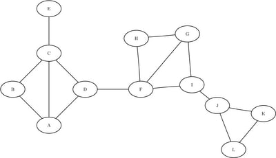
, and ![]() . The induced subgraphs on these three sets of nodes are shown in blue in Figure 1.36 through Figure 1.38. Notice that links that connect different partitions have been removed.
. The induced subgraphs on these three sets of nodes are shown in blue in Figure 1.36 through Figure 1.38. Notice that links that connect different partitions have been removed.
Figure 1.36: Subgraph ![]()
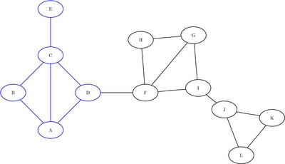
Figure 1.37: Subgraph ![]()
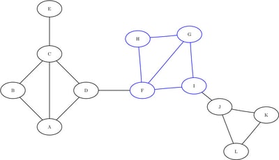
Figure 1.38: Subgraph ![]()
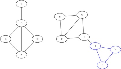
The following data sets define the three induced subgraphs:
data LinkSetIn0;
   input from $ to $ @@;
   datalines;
A B  A C  A D  B C  C D  C E
;

data LinkSetIn1;
   input from $ to $ @@;
   datalines;
F G  F H  F I  G H  G I
;

data LinkSetIn2;
   input from $ to $ @@;
   datalines;
J K  J L  K L
;
To calculate centrality metrics on the three subgraphs, you could run PROC OPTGRAPH three times, as follows:
proc optgraph
   data_links = LinkSetIn0
   out_nodes  = NodeSetOut0;
   centrality
      degree    = out
      influence = unweight
      close     = unweight
      between   = unweight
      eigen     = unweight;
run;

proc optgraph
   data_links = LinkSetIn1
   out_nodes  = NodeSetOut1;
   centrality
      degree    = out
      influence = unweight
      close     = unweight
      between   = unweight
      eigen     = unweight;
run;
proc optgraph
   data_links = LinkSetIn2
   out_nodes  = NodeSetOut2;
   centrality
      degree    = out
      influence = unweight
      close     = unweight
      between   = unweight
      eigen     = unweight;
run;
This produces the results shown in Figure 1.39 through Figure 1.41.
Figure 1.39: Centrality for Induced Subgraph 0
Figure 1.40: Centrality for Induced Subgraph 1
Figure 1.41: Centrality for Induced Subgraph 2
A much more efficient way to process these graphs is to define the partition by using the cluster variable in the nodes data set and using the BY_CLUSTER option. Define the partitions of the original graph as follows:
data NodeSetIn;
   input node $ cluster @@;
   datalines;
A 0  B 0  C 0  D 0  E 0
F 1  G 1  H 1  I 1
J 2  K 2  L 2
;
Now, using one call to PROC OPTGRAPH, you can process all three induced subgraphs. In addition, because the processing of these subgraphs is completely independent, you can do the processing in parallel by using the NTHREADS= option in the PERFORMANCE statement.
proc optgraph
   loglevel     = moderate
   data_nodes   = NodeSetIn
   data_links   = LinkSetIn
   out_nodes    = NodeSetOut;
   performance
      nthreads  = 3;
   centrality
      by_cluster
      degree    = out
      influence = unweight
      close     = unweight
      between   = unweight
      eigen     = unweight;
run;
%put &_OPTGRAPH_;
%put &_OPTGRAPH_CENTRALITY_;
Assuming that your machine has at least three cores, all three subgraphs are processed simultaneously with one call to PROC OPTGRAPH. The progress of the procedure is shown in Figure 1.42.
Figure 1.42: PROC OPTGRAPH Log: Centrality by Cluster for a Simple Undirected Graph
| NOTE: ------------------------------------------------------------------------------------------ |
| NOTE: ------------------------------------------------------------------------------------------ |
| NOTE: Running OPTGRAPH version 14.1. |
| NOTE: ------------------------------------------------------------------------------------------ |
| NOTE: ------------------------------------------------------------------------------------------ |
| NOTE: The OPTGRAPH procedure is executing in single-machine mode. |
| NOTE: ------------------------------------------------------------------------------------------ |
| NOTE: ------------------------------------------------------------------------------------------ |
| NOTE: Reading the nodes data set. |
| NOTE: There were 12 observations read from the data set WORK.NODESETIN. |
| NOTE: Reading the links data set. |
| NOTE: There were 16 observations read from the data set WORK.LINKSETIN. |
| NOTE: Data input used 0.01 (cpu: 0.00) seconds. |
| NOTE: Building the input graph storage used 0.00 (cpu: 0.00) seconds. |
| NOTE: The input graph storage is using 0.3 MBs of memory. |
| NOTE: The number of nodes in the input graph is 12. |
| NOTE: The number of links in the input graph is 16. |
| NOTE: ------------------------------------------------------------------------------------------ |
| NOTE: ------------------------------------------------------------------------------------------ |
| NOTE: Processing centrality metrics by cluster. |
| NOTE: ------------------------------------------------------------------------------------------ |
| NOTE: Using the CLUSTER variable from the DATA_NODES= data set to partition the graph. |
| NOTE: Links that cross subgraphs are ignored. |
| NOTE: ------------------------------------------------------------------------------------------ |
| NOTE: Distribution of 3 subgraphs by number of nodes: |
| 3 subgraphs of size [ 3, 10] (100.0%) |
| NOTE: ------------------------------------------------------------------------------------------ |
| NOTE: Processing centrality metrics by cluster using 3 threads. |
| Cpu Real |
| Algorithm SubGraphs Complete Time Time |
| centrality 3 100% 0.02 0.00 |
| NOTE: Processing centrality metrics used 0.5 MBs of memory. |
| NOTE: Processing centrality metrics by cluster used 0.00 (cpu: 0.02) seconds. |
| NOTE: ------------------------------------------------------------------------------------------ |
| NOTE: ------------------------------------------------------------------------------------------ |
| NOTE: Creating nodes data set output. |
| NOTE: Data output used 0.00 (cpu: 0.00) seconds. |
| NOTE: ------------------------------------------------------------------------------------------ |
| NOTE: ------------------------------------------------------------------------------------------ |
| NOTE: The data set WORK.NODESETOUT has 12 observations and 8 variables. |
| STATUS=OK CENTRALITY=OK |
| STATUS=OK CPU_TIME=0.02 REAL_TIME=0.00 |
The results are shown in Figure 1.43.
Figure 1.43: Centrality for All Induced Subgraphs
| node | cluster | centr_degree_out | centr_eigen_unwt | centr_close_unwt | centr_between_unwt | centr_influence1_unwt | centr_influence2_unwt |
|---|---|---|---|---|---|---|---|
| A | 0 | 3 | 0.89897 | 0.80000 | 0.08333 | 0.60000 | 1.60000 |
| B | 0 | 2 | 0.70711 | 0.66667 | 0.00000 | 0.40000 | 1.40000 |
| C | 0 | 4 | 1.00000 | 1.00000 | 0.58333 | 0.80000 | 1.60000 |
| D | 0 | 2 | 0.70711 | 0.66667 | 0.00000 | 0.40000 | 1.40000 |
| E | 0 | 1 | 0.37236 | 0.57143 | 0.00000 | 0.20000 | 0.80000 |
| F | 1 | 3 | 1.00000 | 1.00000 | 0.16667 | 0.75000 | 1.75000 |
| G | 1 | 3 | 1.00000 | 1.00000 | 0.16667 | 0.75000 | 1.75000 |
| H | 1 | 2 | 0.78078 | 0.75000 | 0.00000 | 0.50000 | 1.50000 |
| I | 1 | 2 | 0.78078 | 0.75000 | 0.00000 | 0.50000 | 1.50000 |
| J | 2 | 2 | 1.00000 | 1.00000 | 0.00000 | 0.66667 | 1.33333 |
| K | 2 | 2 | 1.00000 | 1.00000 | 0.00000 | 0.66667 | 1.33333 |
| L | 2 | 2 | 1.00000 | 1.00000 | 0.00000 | 0.66667 | 1.33333 |
Centrality by Community for a Simple Undirected Graph
The partition defined in the data set NodeSetIn could have also been calculated by PROC OPTGRAPH using a method called community detection. This method is discussed in the section Community. First, call the community detection method as follows:
proc optgraph
   data_links = LinkSetIn
   out_nodes  = Communities;
   community;
run;
The resulting output is a partition of the nodes of the original graph into communities. The data set Communities is shown in Figure 1.44.
Figure 1.44: Communities for a Simple Undirected Graph
To calculate centrality by induced subgraph, you can simply use the communities output as the nodes data set input and use the DATA_NODES_VAR statement to define the cluster variable:
proc optgraph
   data_nodes   = Communities
   data_links   = LinkSetIn
   out_nodes    = NodeSetOut;
   data_nodes_var
      cluster   = community_1;
   performance
      nthreads  = 3;
   centrality
      by_cluster
      degree    = out
      influence = unweight
      close     = unweight
      between   = unweight
      eigen     = unweight;
run;
This gives the same results as before, when you manually defined the partition. These results are shown in Figure 1.43.
Centrality by Filtered Community for a Simple Undirected Graph
In some situations, the community detection algorithm might find a large number of small communities. Those communities might not be relevant, and you might want to focus only on communities of a certain size. When you use the BY_CLUSTER option, you can also use the FILTER_SUBGRAPH= option to ignore any subgraph whose number of nodes is less than or equal to a certain size. This can save on computation time, and the resulting output contains only the subgraphs of interest.
Returning to the data in the section Centrality by Community for a Simple Undirected Graph, you can use the filtering option as follows:
proc optgraph
   filter_subgraph = 3
   data_nodes      = Communities
   data_links      = LinkSetIn
   out_nodes       = NodeSetOut;
   data_nodes_var
      cluster      = community_1;
   performance
      nthreads     = 3;
   centrality
      by_cluster
      degree       = out
      influence    = unweight
      close        = unweight
      between      = unweight
      eigen        = unweight;
run;
The results, shown in Figure 1.45, now contain only those subgraphs with node size greater than 3.
Figure 1.45: Centrality for Some Induced Subgraphs
| node | community_1 | centr_degree_out | centr_eigen_unwt | centr_close_unwt | centr_between_unwt | centr_influence1_unwt | centr_influence2_unwt |
|---|---|---|---|---|---|---|---|
| A | 0 | 3 | 0.89897 | 0.80000 | 0.08333 | 0.60 | 1.60 |
| B | 0 | 2 | 0.70711 | 0.66667 | 0.00000 | 0.40 | 1.40 |
| C | 0 | 4 | 1.00000 | 1.00000 | 0.58333 | 0.80 | 1.60 |
| D | 0 | 2 | 0.70711 | 0.66667 | 0.00000 | 0.40 | 1.40 |
| E | 0 | 1 | 0.37236 | 0.57143 | 0.00000 | 0.20 | 0.80 |
| F | 1 | 3 | 1.00000 | 1.00000 | 0.16667 | 0.75 | 1.75 |
| G | 1 | 3 | 1.00000 | 1.00000 | 0.16667 | 0.75 | 1.75 |
| H | 1 | 2 | 0.78078 | 0.75000 | 0.00000 | 0.50 | 1.50 |
| I | 1 | 2 | 0.78078 | 0.75000 | 0.00000 | 0.50 | 1.50 |