The OPTGRAPH Procedure
- Overview
-
Getting Started

-
SyntaxFunctional SummaryPROC OPTGRAPH StatementBICONCOMP StatementCENTRALITY StatementCLIQUE StatementCOMMUNITY StatementCONCOMP StatementCORE StatementCYCLE StatementDATA_LINKS_VAR StatementDATA_MATRIX_VAR StatementDATA_NODES_VAR StatementEIGENVECTOR StatementLINEAR_ASSIGNMENT StatementMINCOSTFLOW StatementMINCUT StatementMINSPANTREE StatementPERFORMANCE StatementREACH StatementSHORTPATH StatementSUMMARY StatementTRANSITIVE_CLOSURE StatementTSP Statement
-
DetailsGraph Input DataMatrix Input DataData Input OrderParallel ProcessingNumeric LimitationsSize LimitationsCommon Notation and AssumptionsBiconnected Components and Articulation PointsCentralityCliqueCommunityConnected ComponentsCore DecompositionCycleEigenvector ProblemLinear Assignment (Matching)Minimum-Cost Network FlowMinimum CutMinimum Spanning TreeReach (Ego) NetworkShortest PathSummaryTransitive ClosureTraveling Salesman ProblemMacro VariablesODS Table Names
-
ExamplesArticulation Points in a Terrorist NetworkInfluence Centrality for Project Groups in a Research DepartmentBetweenness and Closeness Centrality for Computer Network TopologyBetweenness and Closeness Centrality for Project Groups in a Research DepartmentEigenvector Centrality for Word Sense DisambiguationCentrality Metrics for Project Groups in a Research DepartmentCommunity Detection on Zachary’s Karate Club DataRecursive Community Detection on Zachary’s Karate Club DataCycle Detection for Kidney Donor ExchangeLinear Assignment Problem for Minimizing Swim TimesLinear Assignment Problem, Sparse Format versus Dense FormatMinimum Spanning Tree for Computer Network TopologyTransitive Closure for Identification of Circular Dependencies in a Bug Tracking SystemReach Networks for Computation of Market Coverage of a Terrorist NetworkTraveling Salesman Tour through US Capital Cities
- References
Community
Community detection partitions a graph into communities such that the links within the community subgraphs are more densely connected than the links between communities.
In PROC OPTGRAPH, community detection can be determined by using the COMMUNITY statement. The options for this statement are described in the section COMMUNITY Statement.
The COMMUNITY statement reports status information in a macro variable called _OPTGRAPH_COMMUNITY_. See the section Macro Variable _OPTGRAPH_COMMUNITY_ for more information about this macro variable.
When you specify ALGORITHM= PARALLEL_LABEL_PROP in the COMMUNITY statement, community detection supports both undirected and directed graphs. When you specify ALGORITHM=LOUVAIN or ALGORITHM=LABEL_PROP in the COMMUNITY statement, community detection is supported only for undirected graphs. For directed graphs, you need to aggregate directed links into undirected links before you call the algorithm. For example, suppose there are two directed links: a link from i to j with a link weight of 4.3, and a link from j to i with a link weight of 3.2. One common aggregation strategy is to sum the link weights together. Using this strategy, the weight of the undirected link between i and j is 7.5.
PROC OPTGRAPH implements three heuristic algorithms for finding communities: the LOUVAIN algorithm proposed in Blondel et al. (2008), the label propagation algorithm proposed in Raghavan, Albert, and Kumara (2007), and the parallel label propagation algorithm developed by SAS (patent pending).
Given a graph ![]() , all three algorithms run in time
, all three algorithms run in time ![]() , where k is the average number of links per node. The Louvain algorithm aims to optimize modularity, which is one of the most popular
merit functions for community detection. Modularity is a measure of the quality of a division of a graph into communities.
The modularity of a division is defined to be the fraction of the links that fall within the communities minus the expected fraction if
the links were distributed at random, assuming that you do not change the degree of each node.
, where k is the average number of links per node. The Louvain algorithm aims to optimize modularity, which is one of the most popular
merit functions for community detection. Modularity is a measure of the quality of a division of a graph into communities.
The modularity of a division is defined to be the fraction of the links that fall within the communities minus the expected fraction if
the links were distributed at random, assuming that you do not change the degree of each node.
Mathematically, modularity is defined as
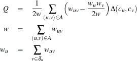
where Q is the modularity, ![]() is the link weight between node u and v,
is the link weight between node u and v, ![]() is the set of nodes that connects to node u,
is the set of nodes that connects to node u, ![]() is the sum of link weights incident to node u, w is the sum of link weights of the graph,
is the sum of link weights incident to node u, w is the sum of link weights of the graph, ![]() is the community to which node u belongs, and
is the community to which node u belongs, and ![]() is the Kronecker delta symbol, defined as
is the Kronecker delta symbol, defined as
The following is a brief description of the Louvain algorithm:
-
Initialize each node as its own community.
-
Move each node from its current community to the neighboring community that increases modularity the most. Repeat this step until modularity cannot be improved.
-
Group the nodes in each community into a supernode. Construct a new graph based on supernodes. Repeat these steps until modularity cannot be further improved or the maximum number of iterations has been reached.
The more recently proposed label propagation algorithm moves a node to a community that most of its neighbors belong to. Extensive testing by Lancichinetti and Fortunato (2009) has empirically demonstrated that the label propagation algorithm performs as well as the Louvain method in most cases.
The following is a brief description of the label propagation algorithm:
-
Initialize each node as its own community.
-
Move each node from its current community to the neighboring community that has the maximum sum of link weights to the current node; break ties randomly if necessary. Repeat this step until there are no more movements.
The parallel label propagation algorithm is an extension of the basic label propagation algorithm. During each iteration, rather than updating node labels sequentially, nodes update their labels simultaneously by using the node label information from the previous iteration. In this approach, node labels can be updated in parallel. However, simultaneous updating of this nature often leads to oscillating labels because of the bipartite subgraph structure often present in large graphs. To address this issue, at each iteration the parallel algorithm skips the labeling step at some randomly chosen nodes in order to break the bipartite structure. You can control the random samples that the algorithm takes by specifying the RANDOM_FACTOR= or RANDOM_SEED= options in the COMMUNITY statement.
As you can see from their descriptions, all three algorithms adopt a heuristic local optimization approach. The final result often depends on the sequence of nodes that are presented in the links input data set. Therefore, if the sequence of nodes in the links data set has been changed, the result is likely to be slightly different.
Parallel Community Detection
Parallel community detection can be invoked by specifying ALGORITHM= PARALLEL_LABEL_PROP in the COMMUNITY statement. The computation is executed with multiple threads on a single computer. The number of threads being used can be controlled by specifying the NTHREADS= option in the PERFORMANCE statement.
The following statements demonstrate how to invoke parallel community detection using eight threads:
proc optgraph
   data_links       = links
   graph_direction  = directed
   out_nodes        = outNodes;
   performance
      nthreads      = 8;
   community
      algorithm     = parallel_label_prop
      out_community = outComm;
run;
Memory Requirement
When you specify GRAPH_INTERNAL_FORMAT=THIN in the PROC OPTGRAPH statement and ALGORITHM=LOUVAIN or ALGORITHM=LABEL_PROP in
the COMMUNITY statement, the memory (number of bytes) required for community detection can be estimated approximately as follows
given a graph ![]() :
:
When you specify GRAPH_INTERNAL_FORMAT=THIN and ALGORITHM=PARALLEL_LABEL_PROP, the memory required for community detection is approximately twice this amount.
Assume that your machine architecture is such that an integer is 4 bytes and a double is 8 bytes. Then, a graph with 100 million nodes and 650 million links would require approximately 21 gigabytes (GB) of memory when you specify ALGORITHM=LOUVAIN or ALGORITHM=LABEL_PROP:
The same graph would require approximately 42 GB if you specify ALGORITHM=PARALLEL_LABEL_PROP.
This is only an estimate for the amount of memory that is required. PROC OPTGRAPH itself might require more memory to maintain the input and output data structures. In addition, other running processes might take away from the available memory.
PROC OPTGRAPH uses significantly more memory if GRAPH_INTERNAL_FORMAT=FULL. It is recommended that you use GRAPH_INTERNAL_FORMAT=THIN when you apply community detection on large graphs.
Graph Direction
If you specify ALGORITHM=PARALLEL_LABEL_PROP in the COMMUNITY statement, community detection supports both undirected and directed graphs. However, you should be careful in deciding whether to model your problem as an undirected or a directed graph. For an undirected graph, the algorithm finds communities based on the density of the subgraphs. For a directed graph, the algorithm finds communities based on the information flow along the directed links. That is, the algorithm propagates the community ID along the outgoing links of a node. Therefore, nodes are likely to be in the same community if they form circles along the outgoing links. If the directed graph lacks this circle structure, the nodes are likely to switch between communities during the computation. As a result, the algorithm does not converge well and cannot find a good community structure in the graph.
Large Community
It has often been observed in practice that the number of nodes contained in communities (produced by community detection algorithms) usually follows a power law distribution. That is, a few communities contain a very large number of nodes, whereas most communities contain a small number of nodes. This is especially true for large graphs. PROC OPTGRAPH provides two approaches to alleviate this problem: one uses the RECURSIVE option, and the other uses the RESOLUTION_LIST= option.
Recursive
You can apply the RECURSIVE option to recursively break large communities into smaller ones. At the first step, PROC OPTGRAPH processes data as if no RECURSIVE option were specified. At the end of this step, it checks whether the community result satisfies the RECURSIVE option criteria. If the community result satisfies these criteria, PROC OPTGRAPH stops iterations and outputs results. Otherwise, it treats each large community as an independent graph and recursively applies community detection on top of it.
In certain cases, a community is not further split even if it does not meet the recursive criteria that you specified. One example is a star-shaped community that contains 200 nodes while MAX_COMM_SIZE is specified as 100; another example is a symmetric community whose diameter is 2 while MAX_DIAMETER is specified as 1.
Resolution List
The second way to combat the problem, provided you have specified ALGORITHM= LOUVAIN in the COMMUNITY statement, is to assign a larger value than the default value of 1 to the RESOLUTION_LIST= option. When ALGORITHM=LOUVAIN, the value assigned to the RESOLUTION_LIST= option can be interpreted as follows: Suppose the resolution value is x. Two communities are merged if the sum of the weights of intercommunity links is at least x times the expected value of the same sum if the graph is reconfigured randomly. Therefore, a larger resolution value produces more communities, each of which contains a smaller number of nodes. However, there is no explicit formula to detail the number of nodes in communities with respect to the resolution value. You must use trial and error to get to the expected community size. More information about resolution value is available in Ronhovde and Nussinov 2010.
If you specify ALGORITHM=LOUVAIN, you can supply multiple resolution values at one time. If you supply multiple resolution values at one time, PROC OPTGRAPH detects communities at the highest resolution level first, then merges communities at a lower resolution, and repeats the process until it reaches the lowest level. This process enables you to see how the communities are merged at different levels. Due to the local nature of this optimization algorithm, two different runs do not produce the same result if the two runs share a common resolution level. For example, the algorithm can produce different results at resolution 0.5 in two runs: one with RESOLUTION_LIST = 1 0.7 0.5, and the other with RESOLUTION_LIST = 1 0.5.
If you specify ALGORITHM=PARALLEL_LABEL_PROP in the COMMUNITY statement, the resolution value can be interpreted as the minimal density of communities in an undirected and unweighted graph. The density of a community is defined as the number of links inside the community divided by the total number of possible links. A larger resolution value likely results in communities that contain fewer nodes. For more information about resolution values for label propagation, see Traag, Van Dooren, and Nesterov (2011).
If you supply multiple resolution values at one time and you specify ALGORITHM=PARALLEL_LABEL_PROP, the OPTGRAPH procedure performs community detection multiple times, each time with a different resolution value. This is equivalent to calling the OPTGRAPH procedure several times, each time with a different (single) resolution value specified for the RESOLUTION_LIST= option.
If you specify ALGORITHM=PARALLEL_LABEL_PROP in the COMMUNITY statement, the value that is specified in the RESOLUTION_LIST= option has a major impact on the running time of the algorithm. When a large resolution value is specified, the algorithm is likely to create many tiny communities, and nodes are likely to change communities between iterations. Therefore, the algorithm might not converge properly. On the other hand, when the resolution value is small, the algorithm might find some very large communities, such as a community that contains more than a million nodes. In this case, if you specify the RECURSIVE option, the algorithm spends a long time in the recursive step in order to break large communities into smaller ones.
The recommended approach is to first experiment with a set of resolution values without using the RECURSIVE option. At the end of the run, examine the resulting modularity values and the community size distributions. Remove the resolution values that lead to small modularity values or huge communities. Then add the RECURSIVE option to the COMMUNITY statement, if desired, and run PROC OPTGRAPH again.
Community Detection on Zachary’s Karate Club Data shows the use of the RESOLUTION_LIST= option in the calculation of communities.
Large Graphs
When you are dealing with large graphs, the following practices are recommended:
-
Use GRAPH_INTERNAL_FORMAT=THIN instead of GRAPH_INTERNAL_FORMAT=FULL. This enables PROC OPTGRAPH to store the data in memory compactly.
-
Use the LINK_REMOVAL_RATIO= option to remove unimportant links. This practice can often dramatically improve the running time of large graphs.
Output Data Sets
Community detection produces up to five output data sets. In these data sets, if you specify ALGORITHM=LOUVAIN or ALGORITHM=LABEL_PROP in the COMMUNITY statement, resolution level numbers are in decreasing order of the values that are specified in the RESOLUTION_LIST= option. That is, resolution level 1 corresponds to the largest value specified in the RESOLUTION_LIST= option, and resolution level K corresponds to the smallest value specified in the RESOLUTION_LIST= option. For example, if RESOLUTION_LIST=2.5 3.1 0.6, then resolution level 1 is at value 3.1, resolution level 2 is at value 2.5, and resolution level 3 is at value 0.6.
If you specify ALGORITHM=PARALLEL_LABEL_PROP in the COMMUNITY statement, resolution level numbers are in the same order as the values that are specified in the RESOLUTION_LIST= option. For example, if RESOLUTION_LIST=0.001 0.005 0.01, then resolution level 1 is at value 0.001, resolution level 2 is at value 0.005, and resolution level 3 is at value 0.01.
OUT_NODES= Data Set
This data set describes the community identifier of each node. If multiple resolution values have been specified, the data set reports the community identifier of each node at each resolution level. The data set contains the following columns:
-
node: node label -
community_i: community identifier at resolution level i, where i is the resolution level number as previously described. There are K such columns if K different values are specified in the RESOLUTION_LIST= option.
OUT_LEVEL= Data Set
This data set describes the number of communities and their corresponding modularity values at various resolution levels. It contains the following columns:
-
level: resolution level number -
resolution: resolution value -
communities: number of communities at the current resolution level -
modularity: modularity value at the current resolution level
OUT_COMMUNITY= Data Set
This data set describes the number of nodes in each community. It contains the following columns:
-
level: resolution level number -
resolution: resolution value -
community: community identifier -
nodes: number of nodes contained in the community
OUT_OVERLAP= Data Set
This data set describes the intensity of each node. At the end of community detection, a node could have links that connect to multiple communities. The intensity of a node is computed as the sum of the link weights that connect to nodes in the specified community divided by the total link weights of the node. This data set is computationally expensive to produce, and it requires a large amount of disk space. Therefore, this data set is not produced if you specify multiple resolution values in the RESOLUTION_LIST= option and ALGORITHM=PARALLEL_LABEL_PROP. However, if ALGORITHM=LOUVAIN, the data set is produced and will only contain results corresponding to the smallest value of the RESOLUTION_LIST= option. The data set contains the following columns:
-
node: node label -
community: community identifier -
intensity: intensity of the node that belongs to the community
OUT_COMM_LINKS= Data Set
This data set describes how communities are connected. If you specify ALGORITHM=LOUVAIN or ALGORITHM=LABEL_PROP in the COMMUNITY statement, this data set contains the following columns:
-
level: resolution level number -
resolution: resolution value -
from_community: community identifier of the from community -
to_community: community identifier of the to community -
link_weight: sum of link weights of all links betweenfrom_communityandto_community
If you specify ALGORITHM=PARALLEL_LABEL_PROP in the COMMUNITY statement, this data set contains the from, to, and link_weight columns. This data set is not produced if you specify ALGORITHM=PARALLEL_LABEL_PROP together with multiple resolution values
in the RESOLUTION_LIST= option.
Community Detection on a Simple Graph
This section illustrates the use of the community detection algorithm on the simple undirected graph G that is shown in Figure 1.51.
Figure 1.51: A Simple Undirected Graph G
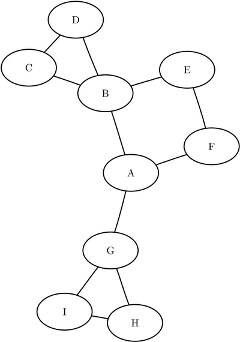
The undirected graph G can be represented by the following links data set LinkSetIn:
data LinkSetIn;
   input from $ to $ @@;
   datalines;
A B  A F  A G  B C  B D
B E  C D  E F  G I  G H
H I
;
The following statements perform community detection and output the results in the specified data sets. The Louvain algorithm is used by default because no value is specified for the ALGORITHM= option.
proc optgraph
   data_links   = LinkSetIn
   out_nodes    = NodeSetOut;
   community
      resolution_list = 1.0 0.5
      out_level       = CommLevelOut
      out_community   = CommOut
      out_overlap     = CommOverlapOut
      out_comm_links  = CommLinksOut;
run;
The data set NodeSetOut contains the community identifier of each node and is shown in Figure 1.52.
Figure 1.52: Community Detection on a Simple Graph: Nodes Output
The data set CommLevelOut contains summary information at each resolution level and is shown in Figure 1.53.
Figure 1.53: Community Detection on a Simple Graph: Level Output
The data set CommOut contains the number of nodes in each community and is shown in Figure 1.54.
Figure 1.54: Community Detection on a Simple Graph: Community Summary
The data set CommOverlapOut contains community overlap information and is shown in Figure 1.55.
Figure 1.55: Community Detection on a Simple Graph: Community Overlap
The data set CommLinksOut describes how the communities are connected and is shown in Figure 1.56.
Figure 1.56: Community Detection on a Simple Graph: Intercommunity Links