The VARMAX Procedure
- Overview
-
Getting Started

-
Syntax
-
DetailsMissing ValuesVARMAX ModelDynamic Simultaneous Equations ModelingImpulse Response FunctionForecastingTentative Order SelectionVAR and VARX ModelingSeasonal Dummies and Time TrendsBayesian VAR and VARX ModelingVARMA and VARMAX ModelingModel Diagnostic ChecksCointegrationVector Error Correction ModelingI(2) ModelVector Error Correction Model in ARMA FormMultivariate GARCH ModelingOutput Data SetsOUT= Data SetOUTEST= Data SetOUTHT= Data SetOUTSTAT= Data SetPrinted OutputODS Table NamesODS GraphicsComputational Issues
-
Examples
- References
COINTEG Statement
-
COINTEG RANK=number <options> ;
The COINTEG statement fits the vector error correction model to the data, tests the restrictions of the long-run parameters and the adjustment parameters, and tests for weak exogeneity in the long-run parameters. The P= option in the MODEL statement specifies the autoregressive order of the VECM. Only one COINTEG statement is allowed.
The cointegrated system uses maximum likelihood estimation. If there are no moving average (MA) terms specified by the Q= option in the MODEL statement, no GARCH terms specified in the GARCH statement, and no general restrictions specified in the BOUND and RESTRICT statements, then PROC VARMAX applies the maximum likelihood analysis proposed by Johansen and Juselius (1990); Johansen (1995a, 1995b). Otherwise, the likelihood is maximized using an optimizer whose options can be specified in the NLOPTIONS statement.
The following statements fit a VECM(2):
proc varmax data=one;
   model y1-y3 / p=2;
   cointeg rank=1;
run;
To test restrictions on  and
and  , you specify the J= option and the H= option, respectively. You specify the EXOGENEITY option in the COINTEG statement for
tests of weak exogeneity in the long-run parameters.
, you specify the J= option and the H= option, respectively. You specify the EXOGENEITY option in the COINTEG statement for
tests of weak exogeneity in the long-run parameters.
The following example of the COINTEG statement specifies tests of restrictions on and , along with tests of weak exogeneity:
proc varmax data=one;
   model y1-y3 / p=2;
   cointeg rank=1 h=(1 0, -1 0, 0 1)
           j=(1 0, 0 0, 0 1) exogeneity;
run;
You must specify the following option:
You can also specify the following options in the COINTEG statement:
- ECTREND
-
specifies the restriction on the drift in the VECM. This option is used in the following cases:
-
There is no separate drift in the VECM, but a constant enters only through the error correction term. For example, for VECM(p),
![\[ \Delta \mb{y} _ t = \balpha (\bbeta ’, \bbeta _0)(\mb{y} _{t-1}’,1)’ + \sum _{i=1}^{p-1} \Phi ^*_ i \Delta \mb{y} _{t-i} + \bepsilon _ t \]](images/etsug_varmax0120.png)
An example of the ECTREND option follows:
model y1 y2 / p=2;
cointeg rank=1 ectrend;
-
There is a separate drift and no separate linear trend in the VECM, but a linear trend enters only through the error correction term. For example, for VECM(p),
![\[ \Delta \mb{y} _ t = \balpha (\bbeta ’, \bbeta _1)(\mb{y} _{t-1}’,t)’ + \sum _{i=1}^{p-1} \Phi ^*_ i \Delta \mb{y} _{t-i} + \bdelta _0 + \bepsilon _ t \]](images/etsug_varmax0121.png)
An example of the ECTREND option with the TREND= option follows:
model y1 y2 / p=2 trend=linear;
cointeg rank=1 ectrend;
If you specify both this option and the NSEASON option in the MODEL statement, then the NSEASON option is ignored. If you specify the NOINT option in the MODEL statement, then this option is ignored.
-
- EXOGENEITY
-
formulates the likelihood ratio tests for testing weak exogeneity in the long-run parameters. The null hypothesis is that one variable is weakly exogenous for the others.
- H=(matrix)
-
specifies the restrictions
 on the
  or
or  cointegrated coefficient matrix
  such that
  , where is known and
  is unknown. If you do not specify the ECTREND option, then the cointegrated coefficient matrix is the cointegrating matrix and the matrix has dimension
  . If you specify the ECTREND option, then the cointegrated coefficient matrix is the cointegrating matrix stacked with the coefficient row vector
  or
or  for the constant or linear trend in the error correction term, and the matrix has dimension
  . Here k is the number of dependent variables and m is
  , where r is defined in the RANK=r option.
For example, consider a VECM(2) with rank equal to 1 on four dependent variables. Then,
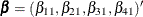 . To test the null hypothesis
  (that is,
  , where
 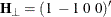 ), you can use the following statements to specify the restriction matrix :
model y1-y4 / p=2;
cointeg rank=1 h=(1 0 0, -1 0 0, 0 1 0, 0 0 1);
Here the dimension of matrix
is  because
  and
and  , and each row of the matrix is separated by commas. Note that
  ; that is, the and
  matrices are orthogonal.
When the series has no separate deterministic trend, and therefore you specify the ECTREND option, the constant term should be restricted by
 . The matrix
  is a
is a  full-rank matrix orthogonal to , such that
 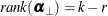 and
and  . The becomes
  or
or 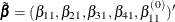 . As for the previous test of (that is,
  , where
 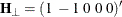 ), you can specify the restriction matrix as follows:
model y1-y4 / p=2;
cointeg rank=1 ectrend
   h=(1 0 0 0, -1 0 0 0, 0 1 0 0, 0 0 1 0, 0 0 0 1);
Because the dimension is changed in the
matrix, the dimension of matrix has to be adjusted accordingly.
When the cointegrated system contains three dependent variables and the RANK=2 option is specified, the test of
 can be run with the following restriction matrix , where
  and :
and :
cointeg rank=2 h=(1 0, -1 0, 0 1);
There are many ways to achieve a matrix that is orthogonal to a particular matrix. The following statements illustrate how to obtain the orthogonal matrix through QR decomposition:
proc iml; /* For a given matrix H_dot, */ H_dot = {1 1 0}`; /* get its QR decomposition, i.e., H_dot = QR. */ call qr(Q, R, piv, lindep, H_dot); /* Then, the matrix orthogonal to H_dot can be extracted from Q. */ H = Q[,ncol(H_dot)+1:nrow(H_dot)]; /* Finally, normalize each column of H if necessary. */ do i = 1 to ncol(H); k = 0; do j = nrow(H) to 1 by -1; if (H[j,i]^=0) then k=j; end; if (k=0) then print "Error: H is not full rank!"; else do j = nrow(H) to 1 by -1; H[j,i] = H[j,i] / H[k,i]; end; end; print "The given matrix is:"; print H_dot; print "The matrix orthogonal to it is:"; print H; quit; - J=(matrix)
-
specifies the restrictions
 on the adjustment matrix such that
  , where is known and
  is unknown. The matrix is specified by using this option, where k is the number of dependent variables, m is , and r is defined in the RANK=r option.
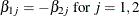
For example, suppose the system contains four variables, the RANK=1 option is specified, and you want to test
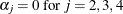 —that is,
  , where
Then you can specify the restriction matrix
as follows:
cointeg rank=1 j=(1, 0, 0, 0);
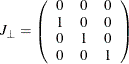
Suppose the system contains three variables, the RANK=2 option is specified, and you want to test
 —that is, , where
  . Then you can specify the restriction matrix as follows:
cointeg rank=2 j=(1 0, 0 0, 0 1);
- NLC
-
specifies the nonlinear constraints that
and are full column rank. Although the constraints are required for a well-defined VECM, only the TECH=QUANEW and TECH=NMSIMP
optimization methods in the NLOPTIONS statement support nonlinear constraints. The full-rank constraints are not imposed by
default so that other optimization methods, such as TECH=CONGRA or TECH=TRUREG, can be tried. The NLC option works only when
numerical optimization is used for estimating VECM (for example, when the BOUND, INITIAL, or RESTRICT statement is specified,
or the VEC-ARMA or VEC-ARMA-GARCH model is estimated). That is, the NLC option is ignored if the closed-form solution of parameter
estimates and maximum likelihood analysis, which is provided in Johansen and Juselius (1990) and Johansen (1995a, 1995b), can be applied.
- NORMALIZE=variable
-
specifies a single dependent (endogenous) variable whose cointegrating vectors are normalized. If the variable is different from the variable specified in the COINTTEST=(JOHANSEN=) or ECM= option in the MODEL statement, the variable in this option is used. If this option is not specified, cointegrating vectors are not normalized.
If the EXOGENEITY, H=, J=, or NORMALIZE= option is specified, the BOUND, GARCH, INITIAL, and RESTRICT statements are all ignored, and the Q= option in the MODEL statement is also ignored.