The VARMAX Procedure
- Overview
-
Getting Started

-
Syntax
-
DetailsMissing ValuesVARMAX ModelDynamic Simultaneous Equations ModelingImpulse Response FunctionForecastingTentative Order SelectionVAR and VARX ModelingSeasonal Dummies and Time TrendsBayesian VAR and VARX ModelingVARMA and VARMAX ModelingModel Diagnostic ChecksCointegrationVector Error Correction ModelingI(2) ModelVector Error Correction Model in ARMA FormMultivariate GARCH ModelingOutput Data SetsOUT= Data SetOUTEST= Data SetOUTHT= Data SetOUTSTAT= Data SetPrinted OutputODS Table NamesODS GraphicsComputational Issues
-
Examples
- References
Example 42.1 Analysis of United States Economic Variables
Consider the following four-dimensional system of US economic variables. Quarterly data for the years 1954 to 1987 are used (Lütkepohl 1993, Table E.3.).
title 'Analysis of US Economic Variables';
data us_money;
   date=intnx( 'qtr', '01jan54'd, _n_-1 );
   format date yyq. ;
   input y1 y2 y3 y4 @@;
   y1=log(y1);
   y2=log(y2);
   label y1='log(real money stock M1)'
         y2='log(GNP in bil. of 1982 dollars)'
         y3='Discount rate on 91-day T-bills'
         y4='Yield on 20-year Treasury bonds';
datalines;
450.9 1406.8  0.010800000 0.026133333
453.0 1401.2 0.0081333333 0.025233333
459.1 1418.0 0.0087000000 0.024900000

   ... more lines ...
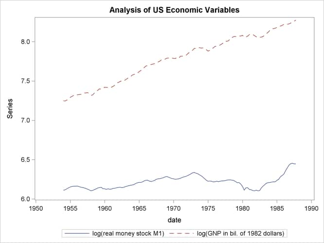
The following statements plot the series:
proc sgplot data=us_money;
   series x=date y=y1 / lineattrs=(pattern=solid);
   series x=date y=y2 / lineattrs=(pattern=dash);
   yaxis label="Series";
run;
Output 42.1.1 shows the plot of the variables  and
and  .
.
Output 42.1.1: Plot of Data
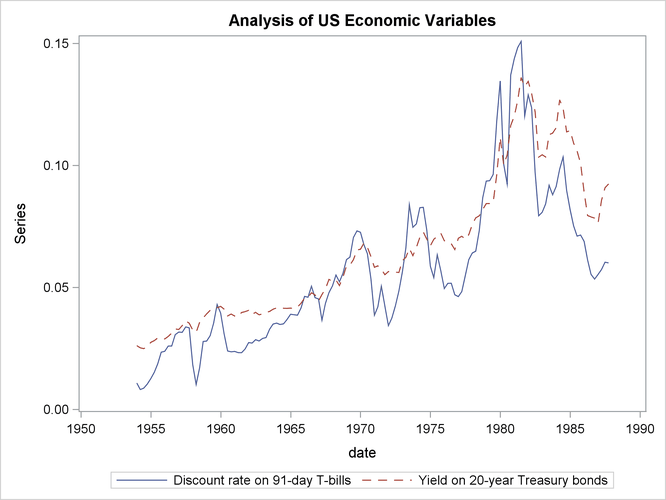
The following statements plot the variables  and
and  :
:
proc sgplot data=us_money;
   series x=date y=y3 / lineattrs=(pattern=solid);
   series x=date y=y4 / lineattrs=(pattern=dash);
   yaxis label="Series";
run;
Output 42.1.2 shows the plot of the variables and .
Output 42.1.2: Plot of Data
The following statements perform the Dickey-Fuller test for stationarity, the Johansen cointegrated test integrated order 2, and the exogeneity test. The VECM(2) is fit to the data.
proc varmax data=us_money;
   id date interval=qtr;
   model y1-y4 / p=2 lagmax=6 dftest
                 print=(iarr(3) estimates diagnose)
                 cointtest=(johansen=(iorder=2));
   cointeg rank=1 normalize=y1 exogeneity;
run;
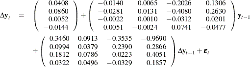
From the outputs shown in Output 42.1.5, you can see that the series has unit roots and is cointegrated in rank 1 with integrated order 1. The fitted VECM(2) is given as
The  prefixed to a variable name implies differencing.
Output 42.1.3 through Output 42.1.16 show the details. Output 42.1.3 shows the descriptive statistics.
Output 42.1.3: Descriptive Statistics
| Analysis of US Economic Variables |
| Number of Observations | 136 |
|---|---|
| Number of Pairwise Missing | 0 |
| Simple Summary Statistics | |||||||
|---|---|---|---|---|---|---|---|
| Variable | Type | N | Mean | Standard Deviation |
Min | Max | Label |
| y1 | Dependent | 136 | 6.21295 | 0.07924 | 6.10278 | 6.45331 | log(real money stock M1) |
| y2 | Dependent | 136 | 7.77890 | 0.30110 | 7.24508 | 8.27461 | log(GNP in bil. of 1982 dollars) |
| y3 | Dependent | 136 | 0.05608 | 0.03109 | 0.00813 | 0.15087 | Discount rate on 91-day T-bills |
| y4 | Dependent | 136 | 0.06458 | 0.02927 | 0.02490 | 0.13600 | Yield on 20-year Treasury bonds |
Output 42.1.4 shows the output for Dickey-Fuller tests for the nonstationarity of each series. The null hypothesis is that there exists a unit root. All series have a unit root.
Output 42.1.4: Unit Root Tests
| Unit Root Test | |||||
|---|---|---|---|---|---|
| Variable | Type | Rho | Pr < Rho | Tau | Pr < Tau |
| y1 | Zero Mean | 0.05 | 0.6934 | 1.14 | 0.9343 |
| Single Mean | -2.97 | 0.6572 | -0.76 | 0.8260 | |
| Trend | -5.91 | 0.7454 | -1.34 | 0.8725 | |
| y2 | Zero Mean | 0.13 | 0.7124 | 5.14 | 0.9999 |
| Single Mean | -0.43 | 0.9309 | -0.79 | 0.8176 | |
| Trend | -9.21 | 0.4787 | -2.16 | 0.5063 | |
| y3 | Zero Mean | -1.28 | 0.4255 | -0.69 | 0.4182 |
| Single Mean | -8.86 | 0.1700 | -2.27 | 0.1842 | |
| Trend | -18.97 | 0.0742 | -2.86 | 0.1803 | |
| y4 | Zero Mean | 0.40 | 0.7803 | 0.45 | 0.8100 |
| Single Mean | -2.79 | 0.6790 | -1.29 | 0.6328 | |
| Trend | -12.12 | 0.2923 | -2.33 | 0.4170 | |
The Johansen cointegration rank test shows whether the series is integrated order either 1 or 2 as shown in Output 42.1.5. The last two columns in Output 42.1.5 explain the cointegration rank test with integrated order 1. The results indicate that there is a cointegrated relationship
with cointegration rank 1 with respect to the 0.05 significance level because the test statistic for the null hypothesis H0:
 is 55.9633 and its corresponding p-value is 0.0072, less than 0.05 (indicating that H0: should be rejected), and the test statistic for the null hypothesis H0:
  is 20.6542 and its corresponding p-value is 0.3775, greater than 0.05 (indicating that H0: cannot be rejected). Now, look at the row associated with . All p-values of the tests for the null hypothesis that the series are integrated order 2 are zeros, less than 0.05 significance
level (indicating that the null hypothesis should be rejected).
is 20.6542 and its corresponding p-value is 0.3775, greater than 0.05 (indicating that H0: cannot be rejected). Now, look at the row associated with . All p-values of the tests for the null hypothesis that the series are integrated order 2 are zeros, less than 0.05 significance
level (indicating that the null hypothesis should be rejected).
Output 42.1.5: Cointegration Rank Test
| Cointegration Rank Test for I(2) | ||||||
|---|---|---|---|---|---|---|
| r\k-r-s | 4 | 3 | 2 | 1 | Trace of I(1) |
Pr > Trace of I(1) |
| 0 | 384.6090 | 214.3790 | 107.9378 | 37.0252 | 55.9633 | 0.0072 |
| Pr > Trace of I(2) | 0.0000 | 0.0000 | 0.0000 | 0.0000 | ||
| 1 | 219.6239 | 89.2151 | 27.3261 | 20.6542 | 0.3775 | |
| Pr > Trace of I(2) | 0.0000 | 0.0000 | 0.0000 | |||
| 2 | 73.6178 | 22.1328 | 2.6477 | 0.9803 | ||
| Pr > Trace of I(2) | 0.0000 | 0.0000 | ||||
| 3 | 38.2943 | 0.0149 | 0.9031 | |||
| Pr > Trace of I(2) | 0.0000 | |||||
Output 42.1.6 shows the estimates of the long-run parameter,  , and the adjustment coefficient,
  .
.
Output 42.1.6: Cointegration Rank Test, Continued
| Beta | ||||
|---|---|---|---|---|
| Variable | 1 | 2 | 3 | 4 |
| y1 | 1.00000 | 1.00000 | 1.00000 | 1.00000 |
| y2 | -0.46458 | -0.63174 | -0.69996 | -0.16140 |
| y3 | 14.51619 | -1.29864 | 1.37007 | -0.61806 |
| y4 | -9.35520 | 7.53672 | 2.47901 | 1.43731 |
| Alpha | ||||
|---|---|---|---|---|
| Variable | 1 | 2 | 3 | 4 |
| y1 | -0.01396 | 0.01396 | -0.01119 | 0.00008 |
| y2 | -0.02811 | -0.02739 | -0.00032 | 0.00076 |
| y3 | -0.00215 | -0.04967 | -0.00183 | -0.00072 |
| y4 | 0.00510 | -0.02514 | -0.00220 | 0.00016 |
Output 42.1.7 shows the estimates  and
and  .
.
Output 42.1.7: Cointegration Rank Test, Continued
| Eta | ||||
|---|---|---|---|---|
| Variable | 1 | 2 | 3 | 4 |
| y1 | 52.74907 | 41.74502 | -20.80403 | 55.77415 |
| y2 | -49.10609 | -9.40081 | 98.87199 | 22.56416 |
| y3 | 68.29674 | -144.83173 | -27.35953 | 15.51142 |
| y4 | 121.25932 | 271.80496 | 85.85156 | -130.11599 |
| Xi | ||||
|---|---|---|---|---|
| Variable | 1 | 2 | 3 | 4 |
| y1 | -0.00842 | -0.00052 | -0.00208 | -0.00250 |
| y2 | 0.00141 | 0.00213 | -0.00736 | -0.00058 |
| y3 | -0.00445 | 0.00541 | -0.00150 | 0.00310 |
| y4 | -0.00211 | -0.00064 | -0.00130 | 0.00197 |
Output 42.1.8 shows that the VECM(2) is fit to the data. The RANK=1 option in the COINTEG statement produces the estimates of the long-run
parameter, , and the adjustment coefficient, .
Output 42.1.8: Parameter Estimates
Output 42.1.9 shows the parameter estimates in terms of the constant, the lag 1 coefficients ( ) that are contained in the
  estimates, and the coefficients that are associated with the lag 1 first differences (
 ).
).
Output 42.1.9: Parameter Estimates, Continued
| Constant | |
|---|---|
| Variable | Constant |
| y1 | 0.04076 |
| y2 | 0.08595 |
| y3 | 0.00518 |
| y4 | -0.01438 |
| Parameter Alpha * Beta' Estimates | ||||
|---|---|---|---|---|
| Variable | y1 | y2 | y3 | y4 |
| y1 | -0.01396 | 0.00648 | -0.20263 | 0.13059 |
| y2 | -0.02811 | 0.01306 | -0.40799 | 0.26294 |
| y3 | -0.00215 | 0.00100 | -0.03121 | 0.02011 |
| y4 | 0.00510 | -0.00237 | 0.07407 | -0.04774 |
| AR Coefficients of Differenced Lag | |||||
|---|---|---|---|---|---|
| DIF Lag | Variable | y1 | y2 | y3 | y4 |
| 1 | y1 | 0.34603 | 0.09131 | -0.35351 | -0.96895 |
| y2 | 0.09936 | 0.03791 | 0.23900 | 0.28661 | |
| y3 | 0.18118 | 0.07859 | 0.02234 | 0.40508 | |
| y4 | 0.03222 | 0.04961 | -0.03292 | 0.18568 | |
Output 42.1.10 through Output 42.1.12 show the parameter estimates and their significance.
Output 42.1.10: Parameter Estimates, Continued
| Model Parameter Estimates | ||||||
|---|---|---|---|---|---|---|
| Equation | Parameter | Estimate | Standard Error |
t Value | Pr > |t| | Variable |
| D_y1 | CONST1 | 0.04076 | 0.01418 | 2.87 | 0.0048 | 1 |
| AR1_1_1 | -0.01396 | 0.00495 | -2.82 | 0.0056 | y1(t-1) | |
| AR1_1_2 | 0.00648 | 0.00230 | 2.82 | 0.0056 | y2(t-1) | |
| AR1_1_3 | -0.20263 | 0.07191 | -2.82 | 0.0056 | y3(t-1) | |
| AR1_1_4 | 0.13059 | 0.04634 | 2.82 | 0.0056 | y4(t-1) | |
| AR2_1_1 | 0.34603 | 0.06414 | 5.39 | <.0001 | D_y1(t-1) | |
| AR2_1_2 | 0.09131 | 0.07334 | 1.25 | 0.2154 | D_y2(t-1) | |
| AR2_1_3 | -0.35351 | 0.11024 | -3.21 | 0.0017 | D_y3(t-1) | |
| AR2_1_4 | -0.96895 | 0.20737 | -4.67 | <.0001 | D_y4(t-1) | |
| D_y2 | CONST2 | 0.08595 | 0.01679 | 5.12 | <.0001 | 1 |
| AR1_2_1 | -0.02811 | 0.00586 | -4.79 | <.0001 | y1(t-1) | |
| AR1_2_2 | 0.01306 | 0.00272 | 4.79 | <.0001 | y2(t-1) | |
| AR1_2_3 | -0.40799 | 0.08514 | -4.79 | <.0001 | y3(t-1) | |
| AR1_2_4 | 0.26294 | 0.05487 | 4.79 | <.0001 | y4(t-1) | |
| AR2_2_1 | 0.09936 | 0.07594 | 1.31 | 0.1932 | D_y1(t-1) | |
| AR2_2_2 | 0.03791 | 0.08683 | 0.44 | 0.6632 | D_y2(t-1) | |
| AR2_2_3 | 0.23900 | 0.13052 | 1.83 | 0.0695 | D_y3(t-1) | |
| AR2_2_4 | 0.28661 | 0.24552 | 1.17 | 0.2453 | D_y4(t-1) | |
| D_y3 | CONST3 | 0.00518 | 0.01608 | 0.32 | 0.7476 | 1 |
| AR1_3_1 | -0.00215 | 0.00562 | -0.38 | 0.7024 | y1(t-1) | |
| AR1_3_2 | 0.00100 | 0.00261 | 0.38 | 0.7024 | y2(t-1) | |
| AR1_3_3 | -0.03121 | 0.08151 | -0.38 | 0.7024 | y3(t-1) | |
| AR1_3_4 | 0.02011 | 0.05253 | 0.38 | 0.7024 | y4(t-1) | |
| AR2_3_1 | 0.18118 | 0.07271 | 2.49 | 0.0140 | D_y1(t-1) | |
| AR2_3_2 | 0.07859 | 0.08313 | 0.95 | 0.3463 | D_y2(t-1) | |
| AR2_3_3 | 0.02234 | 0.12496 | 0.18 | 0.8584 | D_y3(t-1) | |
| AR2_3_4 | 0.40508 | 0.23506 | 1.72 | 0.0873 | D_y4(t-1) | |
| D_y4 | CONST4 | -0.01438 | 0.00803 | -1.79 | 0.0758 | 1 |
| AR1_4_1 | 0.00510 | 0.00281 | 1.82 | 0.0713 | y1(t-1) | |
| AR1_4_2 | -0.00237 | 0.00130 | -1.82 | 0.0713 | y2(t-1) | |
| AR1_4_3 | 0.07407 | 0.04072 | 1.82 | 0.0713 | y3(t-1) | |
| AR1_4_4 | -0.04774 | 0.02624 | -1.82 | 0.0713 | y4(t-1) | |
| AR2_4_1 | 0.03222 | 0.03632 | 0.89 | 0.3768 | D_y1(t-1) | |
| AR2_4_2 | 0.04961 | 0.04153 | 1.19 | 0.2345 | D_y2(t-1) | |
| AR2_4_3 | -0.03292 | 0.06243 | -0.53 | 0.5990 | D_y3(t-1) | |
| AR2_4_4 | 0.18568 | 0.11744 | 1.58 | 0.1164 | D_y4(t-1) | |
Output 42.1.11: Parameter Estimates, Continued
| Alpha and Beta Parameter Estimates | ||||||
|---|---|---|---|---|---|---|
| Equation | Parameter | Estimate | Standard Error |
t Value | Pr > |t| | Variable |
| D_y1 | ALPHA1_1 | -0.01396 | 0.00495 | -2.82 | 0.0056 | Beta[,1]'*_DEP_(t-1) |
| BETA1_1 | 1.00000 | y1(t-1) | ||||
| D_y2 | ALPHA2_1 | -0.02811 | 0.00586 | -4.79 | <.0001 | Beta[,1]'*_DEP_(t-1) |
| BETA2_1 | -0.46458 | y2(t-1) | ||||
| D_y3 | ALPHA3_1 | -0.00215 | 0.00562 | -0.38 | 0.7024 | Beta[,1]'*_DEP_(t-1) |
| BETA3_1 | 14.51619 | y3(t-1) | ||||
| D_y4 | ALPHA4_1 | 0.00510 | 0.00281 | 1.82 | 0.0713 | Beta[,1]'*_DEP_(t-1) |
| BETA4_1 | -9.35520 | y4(t-1) | ||||
Output 42.1.12: Parameter Estimates, Continued
| Covariance Parameter Estimates | ||||
|---|---|---|---|---|
| Parameter | Estimate | Standard Error |
t Value | Pr > |t| |
| COV1_1 | 0.00005 | 0.00001 | 8.19 | <.0001 |
| COV1_2 | 0.00001 | 0.00001 | 2.78 | 0.0062 |
| COV2_2 | 0.00007 | 0.00001 | 8.19 | <.0001 |
| COV1_3 | -0.00001 | 0.00001 | -1.60 | 0.1118 |
| COV2_3 | 0.00002 | 0.00001 | 2.71 | 0.0077 |
| COV3_3 | 0.00007 | 0.00001 | 8.19 | <.0001 |
| COV1_4 | -0.00000 | 0.00000 | -1.31 | 0.1936 |
| COV2_4 | 0.00001 | 0.00000 | 3.29 | 0.0013 |
| COV3_4 | 0.00002 | 0.00000 | 6.67 | <.0001 |
| COV4_4 | 0.00002 | 0.00000 | 8.19 | <.0001 |
Output 42.1.13 shows the innovation covariance matrix estimates, the log-likelihood, the various information criteria results, and the tests for white noise residuals. According to the Portmanteau test results, the residuals have significant correlations at lag 2 and 3, indicating that a VECM(3) model might be a better fit than the VECM(2) model.
Output 42.1.13: Diagnostic Checks
| Covariances of Innovations | ||||
|---|---|---|---|---|
| Variable | y1 | y2 | y3 | y4 |
| y1 | 0.00005 | 0.00001 | -0.00001 | -0.00000 |
| y2 | 0.00001 | 0.00007 | 0.00002 | 0.00001 |
| y3 | -0.00001 | 0.00002 | 0.00007 | 0.00002 |
| y4 | -0.00000 | 0.00001 | 0.00002 | 0.00002 |
| Log-likelihood | 2479.23 |
|---|
| Information Criteria | |
|---|---|
| AICC | -4859 |
| HQC | -4844.07 |
| AIC | -4886.46 |
| SBC | -4782.14 |
| FPEC | 2.23E-18 |
| Schematic Representation of Cross Correlations of Residuals |
|||||||
|---|---|---|---|---|---|---|---|
| Variable/Lag | 0 | 1 | 2 | 3 | 4 | 5 | 6 |
| y1 | ++.. | .... | ++.. | .... | +... | ..-- | .... |
| y2 | ++++ | .... | .... | .... | .... | .... | .... |
| y3 | .+++ | .... | +.-. | ..++ | -... | .... | .... |
| y4 | .+++ | .... | .... | ..+. | .... | .... | .... |
| + is > 2*std error, - is < -2*std error, . is between | |||||||
| Portmanteau Test for Cross Correlations of Residuals |
|||
|---|---|---|---|
| Up To Lag | DF | Chi-Square | Pr > ChiSq |
| 3 | 16 | 53.90 | <.0001 |
| 4 | 32 | 74.03 | <.0001 |
| 5 | 48 | 103.08 | <.0001 |
| 6 | 64 | 116.94 | <.0001 |
Output 42.1.14 describes how well each univariate equation fits the data. The residuals for and differ from normality. Except for the residuals for , there are no AR effects on other residuals. Except for the residuals for , there are no ARCH effects on other residuals.
Output 42.1.14: Diagnostic Checks, Continued
| Univariate Model ANOVA Diagnostics | ||||
|---|---|---|---|---|
| Variable | R-Square | Standard Deviation |
F Value | Pr > F |
| y1 | 0.6754 | 0.00712 | 32.51 | <.0001 |
| y2 | 0.3070 | 0.00843 | 6.92 | <.0001 |
| y3 | 0.1328 | 0.00807 | 2.39 | 0.0196 |
| y4 | 0.0831 | 0.00403 | 1.42 | 0.1963 |
| Univariate Model White Noise Diagnostics | |||||
|---|---|---|---|---|---|
| Variable | Durbin Watson |
Normality | ARCH | ||
| Chi-Square | Pr > ChiSq | F Value | Pr > F | ||
| y1 | 2.13418 | 7.19 | 0.0275 | 1.62 | 0.2053 |
| y2 | 2.04003 | 1.20 | 0.5483 | 1.23 | 0.2697 |
| y3 | 1.86892 | 253.76 | <.0001 | 1.78 | 0.1847 |
| y4 | 1.98440 | 105.21 | <.0001 | 21.01 | <.0001 |
| Univariate Model AR Diagnostics | ||||||||
|---|---|---|---|---|---|---|---|---|
| Variable | AR1 | AR2 | AR3 | AR4 | ||||
| F Value | Pr > F | F Value | Pr > F | F Value | Pr > F | F Value | Pr > F | |
| y1 | 0.68 | 0.4126 | 2.98 | 0.0542 | 2.01 | 0.1154 | 2.48 | 0.0473 |
| y2 | 0.05 | 0.8185 | 0.12 | 0.8842 | 0.41 | 0.7453 | 0.30 | 0.8762 |
| y3 | 0.56 | 0.4547 | 2.86 | 0.0610 | 4.83 | 0.0032 | 3.71 | 0.0069 |
| y4 | 0.01 | 0.9340 | 0.16 | 0.8559 | 1.21 | 0.3103 | 0.95 | 0.4358 |
The PRINT=(IARR) option provides the VAR(2) representation in Output 42.1.15.
Output 42.1.15: Infinite Order AR Representation
| Infinite Order AR Representation | |||||
|---|---|---|---|---|---|
| Lag | Variable | y1 | y2 | y3 | y4 |
| 1 | y1 | 1.33208 | 0.09780 | -0.55614 | -0.83836 |
| y2 | 0.07125 | 1.05096 | -0.16899 | 0.54955 | |
| y3 | 0.17903 | 0.07959 | 0.99113 | 0.42520 | |
| y4 | 0.03732 | 0.04724 | 0.04116 | 1.13795 | |
| 2 | y1 | -0.34603 | -0.09131 | 0.35351 | 0.96895 |
| y2 | -0.09936 | -0.03791 | -0.23900 | -0.28661 | |
| y3 | -0.18118 | -0.07859 | -0.02234 | -0.40508 | |
| y4 | -0.03222 | -0.04961 | 0.03292 | -0.18568 | |
| 3 | y1 | 0.00000 | 0.00000 | 0.00000 | 0.00000 |
| y2 | 0.00000 | 0.00000 | 0.00000 | 0.00000 | |
| y3 | 0.00000 | 0.00000 | 0.00000 | 0.00000 | |
| y4 | 0.00000 | 0.00000 | 0.00000 | 0.00000 | |
Output 42.1.16 shows whether each variable is the weak exogeneity of other variables. The variable is not the weak exogeneity of other variables, , , and ; the variable is not the weak exogeneity of other variables, , , and ; the variable and are the weak exogeneity of other variables.
Output 42.1.16: Weak Exogeneity Test