The VARMAX Procedure

Example 42.3 Analysis of Restricted Cointegrated Systems

Subsections:

Weak Exogeneity Tests
Identification
Tests for Long-Run Parameter

The structural relationships between economic time series have been of interest for decades. Because of the cointegration, the vector error correction model (VECM), introduced by Engle and Granger (1987), is one of the most important tools for performing such analysis. Although there exist analytical solutions for a nonrestricted VECM and some restricted VECMs in special forms, the estimation of a generally restricted VECM relies on numerical methods. This section illustrates how to use the RESTRICT (or BOUND) and TEST statements, together with the COINTEG statement, to estimate the restricted VECM and perform the statistical tests. For more information about this topic, see Boswijk and Doornik (2004) and references therein.

The data are simulated based on the VECM

$\begin{eqnarray*} \Delta \mb{y} _ t & =& \balpha \bbeta ’\mb{y}_{t-1}+\Phi _1^*\Delta \mb{y}_{t-1} +\Theta _0^*\mb{x}_{t}+ \bepsilon _ t \\ & =& \left[ \begin{array}{rr} 0.01 & -0.02 \\ -0.03 & 0.04 \\ 0.05 & -0.06 \\ 0 & 0 \end{array} \right] \left[ \begin{array}{rrrr} 1 & 0 & -1 & 0 \\ 0 & 1 & 0 & -1 \end{array} \right] \mb{y}_{t-1} \\ & & + \left[ \begin{array}{rrrr} -0.01 & 0.03 & 0.05 & -0.02 \\ 0.02 & -0.04 & 0.06 & 0.03 \\ 0 & 0 & 0.10 & 0 \\ 0 & 0 & 0 & 0.04 \end{array} \right] \Delta \mb{y}_{t-1} + \left[ \begin{array}{r} 0 \\ 0 \\ 0 \\ 0 \end{array} \right] \mb{x}_{t} + \bepsilon _ t, \\ \bepsilon _ t & \sim & \mr{i.i.d.}~ N(0,\Sigma ),\Sigma =I_4 \end{eqnarray*}$

where $I_4$ is the $4 \times 4$ identity matrix.

The following statements implement the simulation:

title 'Analysis of Restricted Cointegrated Systems';
proc iml;
   alpha = {0.01 -0.02, -0.03 0.04, 0.05 -0.06, 0 0};
   beta = {1 0, 0 1, -1 0, 0 -1};
   phiStar = {-0.01  0.03 0.05 -0.02,
               0.02 -0.04 0.06  0.03,
                  0     0 0.10     0,
                  0     0    0  0.04};
   Pi = alpha * beta` ;
   A1 = I(4) + Pi+ phiStar;
   A2 = -phiStar;
   phi = A1 // A2;
   sig = I(4);

   /* to simulate the vector time series */
   T = 600;
   myseed = 2;
   call varmasim(y,phi) sigma=sig n=T seed=myseed;
   x = J(T,1,0);
   do i = 1 to T;
      x[i] = normal(myseed);
   end;
   y = y || x;

   cn = {'y1' 'y2' 'y3' 'y4' 'x'};
   create simul5 from y[colname=cn];
   append from y;
   close;
quit;

Weak Exogeneity Tests

This example shows different methods for checking weak exogeneity.

The first method uses the EXOGENEITY option in the following statements, and the test results are shown in Output 42.3.1.

/* Method 1 -- To use the EXOGENEITY option */
ods output LogLikelihood = tbl_ll_g;
proc varmax data=simul5;
   model y1 y2 y3 y4 = x / noint p=2;
   cointeg rank=2 exogeneity;
run;

Output 42.3.1: Test Weak Exogeneity with the EXOGENEITY Option

Analysis of Restricted Cointegrated Systems

The VARMAX Procedure

Testing Weak Exogeneity of Each Variables
Variable	DF	Chi-Square	Pr > ChiSq
y1	2	102.96	<.0001
y2	2	116.12	<.0001
y3	2	200.80	<.0001
y4	2	3.99	0.1357

The second method uses the RESTRICT statement and then the likelihood ratio (LR) test in the following statements. The results are shown in Output 42.3.2. In theory, the first and second methods should have exactly same statistics and p-values because they implement the same LR tests. However, because of the difference between the analytical solution and the numerical solution for the restricted VECM, the statistics are a little different, although for the 0.05 significance level they lead to the same correct conclusion: the variable $y1$ is not the weak exogeneity of variables $y2$ , $y3$ , and $y4$ ; the variable $y2$ is not the weak exogeneity of variables $y1$ , $y3$ , and $y4$ ; the variable $y3$ is not the weak exogeneity of variables $y1$ , $y2$ , and $y4$ ; the variable $y4$ is the weak exogeneity of variables $y1$ , $y2$ , and $y3$ .

/* Method 2 -- Use the RESTRICT statement and implement LR test */
%macro LRTestForVECM();
   %do i = 1 %to 4;
      ods output LogLikelihood = tbl_ll_r1_&i.;
      proc varmax data=simul5;
         model y1 y2 y3 y4 = x / noint p=2;
         cointeg rank=2;
         restrict alpha(&i.,1:2) = 0;
      run;
   %end;
   proc iml;
      use tbl_ll_g;
      read all var {nValue1} into ll_g;
      close;
      %do i = 1 %to 4;
         use tbl_ll_r1_&i.;
         read all var {nValue1} into ll_r_&i.;
         close;
      %end;
      DF = J(4,1,2);
      ll_r = ll_r_1 // ll_r_2 // ll_r_3 // ll_r_4;
      Stat = -2*(ll_r - ll_g);
      pValue = 1-cdf("CHISQUARE", Stat, DF);
      Test =  {"H0: Alpha(1,)=0"} // {"H0: Alpha(2,)=0"}
           // {"H0: Alpha(3,)=0"} // {"H0: Alpha(4,)=0"};
      print  Test DF Stat pValue;
   quit;
%mend;
%LRTestForVECM();

Output 42.3.2: Test Weak Exogeneity with the RESTRICT Statement and LR Tests

Analysis of Restricted Cointegrated Systems

Test	DF	Stat	pValue
H0: Alpha(1,)=0	2	109.05157	0
H0: Alpha(2,)=0	2	124.56535	0
H0: Alpha(3,)=0	2	238.35505	0
H0: Alpha(4,)=0	2	5.0877699	0.0785606

The third method uses the TEST statement, which implements the Wald tests. Asymptotically, the Wald test has the same distribution as the LR test.

/* Method 3 -- To use the TEST statement and the Wald test */
proc varmax data=simul5;
   model y1 y2 y3 y4 = x / noint p=2;
   cointeg rank=2;
   test alpha(1,1:2) = 0;
   test alpha(2,1:2) = 0;
   test alpha(3,1:2) = 0;
   test alpha(4,1:2) = 0;
run;

Based on the test results shown in Output 42.3.3, the same correct conclusion can be obtained at the 0.05 significance level: the variable $y1$ is not the weak exogeneity of variables $y2$ , $y3$ , and $y4$ ; the variable $y2$ is not the weak exogeneity of variables $y1$ , $y3$ , and $y4$ ; the variable $y3$ is not the weak exogeneity of variables $y1$ , $y2$ , and $y4$ ; the variable $y4$ is the weak exogeneity of variables $y1$ , $y2$ , and $y3$ .

Output 42.3.3: Test Weak Exogeneity with the TEST Statement, Wald Tests

Analysis of Restricted Cointegrated Systems

The VARMAX Procedure

Testing of the Parameters
Test	DF	Chi-Square	Pr > ChiSq
1	2	113.27	<.0001
2	2	129.15	<.0001
3	2	245.21	<.0001
4	2	4.81	0.0903

Identification

This example shows how important it is to identify $\balpha$ and $\bbeta$ when applying the Wald test on $\balpha$ . First, in the following statements, there are no constraints on $\bbeta$ :

proc varmax data=simul5;
   model y1 y2 y3 y4 = x / noint p=2;
   cointeg rank=2;
   test alpha(1,2) = alpha(2,2) + alpha(3,2);
run;

As shown in Output 42.3.4, based on the test results, the null hypothesis H0: $\balpha [1,2] = \balpha [2,2] + \balpha [3,2]$ should be rejected at the 0.05 significance level, although the true parameter values for the data generating process indicate that H0 is correct.

Output 42.3.4: Importance of Identifying $\balpha$ and $\bbeta$ in the Wald Test

Analysis of Restricted Cointegrated Systems

The VARMAX Procedure

Testing of the Parameters
Test	DF	Chi-Square	Pr > ChiSq
1	1	21.44	<.0001

In the following statements, $r^2$ constraints are now imposed on $\bbeta$ , where r is the cointegration rank:

proc varmax data=simul5;
   model y1 y2 y3 y4 = x / noint p=2;
   cointeg rank=2;
   restrict beta(3:4,1:2) = -I(2);
   test alpha(1,2) = alpha(2,2) + alpha(3,2);
run;

As shown in Output 42.3.5, the null hypothesis cannot be rejected at 0.05 significance level; that is to say, the correct conclusion is achieved.

Output 42.3.5: Importance of Identifying $\balpha$ and $\bbeta$ in the Wald Test, Continued

Analysis of Restricted Cointegrated Systems

The VARMAX Procedure

Testing of the Parameters
Test	DF	Chi-Square	Pr > ChiSq
1	1	0.25	0.6157

Besides $\balpha$ , other short-run parameters in a VECM can also be tested by using the TEST statement. Because short-run parameters other than $\balpha$ are identified in a VECM, it is not necessary to impose additional constraints on $\balpha$ and $\bbeta$ . The following statements test the null hypothesis H0: $\Phi _1^*=0$ :

proc varmax data=simul5;
   model y1 y2 y3 y4 = x / noint p=2;
   cointeg rank=2;
   test ar(2);
run;

According to the results shown in Output 42.3.6, the null hypothesis should be rejected at the 0.05 significance level.

Output 42.3.6: Wald Tests for Short-Run Parameters

Analysis of Restricted Cointegrated Systems

The VARMAX Procedure

Testing of the Parameters
Test	DF	Chi-Square	Pr > ChiSq
1	16	32.79	0.0079

The following statements test the null hypothesis H0: $\Theta _0^*=0$ :

proc varmax data=simul5;
   model y1 y2 y3 y4 = x / noint p=2;
   cointeg rank=2;
   test xl;
run;

According to the results shown in Output 42.3.7, the null hypothesis cannot be rejected at the 0.05 significance level.

Output 42.3.7: Wald Tests for Short-Run Parameters, Continued

Analysis of Restricted Cointegrated Systems

The VARMAX Procedure

Testing of the Parameters
Test	DF	Chi-Square	Pr > ChiSq
1	4	6.01	0.1982

Besides the parameters that are estimated in a VECM, you can also use the TEST statement on $\Pi (=\balpha \bbeta ’)$ , and $\bdelta _0$ or $\bdelta _1$ for Case 2 or 4 when the constant or linear trend, respectively, is restricted in the error correction term. However, keep in mind that the covariance matrix for these parameter estimates is singular when the cointegration rank is less than the number of dependent variables; hence, you might not get the results for some tests.

proc varmax data=simul5;
   model y1 y2 y3 y4 = x / noint p=2;
   cointeg rank=2;
   test ar(1,4,1:4);
   test ar(1,4,{1 3});
run;

As shown in Output 42.3.8, the first test on H0: $\Pi [4,]=0$ cannot be calculated, whereas the second test on H0: $\Pi [4,1] = \Pi [4,3] = 0$ can be.

Output 42.3.8: Wald Tests for $\Pi$

Analysis of Restricted Cointegrated Systems

The VARMAX Procedure

Testing of the Parameters
Test	DF	Chi-Square	Pr > ChiSq
1	4
2	2	4.81	0.0903

Tests for Long-Run Parameter

This example focuses on testing the relationships on the long-run parameter $\bbeta$ . Here, only the following specific form of hypothesis is discussed,

$\mr{H0}\colon \bbeta = (\bH , \bphi )$

where $\bH$ is a known $k \times r_1$ matrix, $\bphi$ is a freely varying $k \times (r-r_1)$ parameter matrix, k is the number of dependent variables, r is the cointegration rank, and $0 \leq r_1 \leq r$ . Other forms of hypothesis—for example, H0: 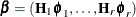$\bbeta = (\bH _1\bphi _1, \ldots , \bH _ r\bphi _ r)$ or H0: $\bH \mr{vec}(\bbeta )=\mb{h}$ —are omitted, although they can also be implemented in the same logic. The following statements test the null hypothesis that $(1~ 0~ -1~ 0)’$ is in the cointegrating space that is spanned by $\bbeta$ :

/* Use the RESTRICT statement and LR test for restrictions on Beta. */
/* H0: Beta = [ H, phi ] where H is known and phi is free */
ods output LogLikelihood = tbl_ll_r2;
proc varmax data=simul5;
   model y1 y2 y3 y4 = x / noint p=2;
   cointeg rank=2;
   restrict beta(,1) = {1, 0, -1, 0};
   nloptions tech=qn maxit=5000;
run;

proc iml;
   use tbl_ll_g;
   read all var {nValue1} into ll_g;
   close;
   use tbl_ll_r2;
   read all var {nValue1} into ll_r;
   close;
   DF = (4-2)*1; /* DF = (k-r)*r_1 */
   Stat = -2*(ll_r - ll_g);
   pValue = 1-cdf("CHISQUARE", stat, df);
   Test = "H0: Beta[1,1:4] = {1 0 -1 0}'";
   print  Test DF Stat pValue;
quit;

According to the result shown in Output 42.3.9, the null hypothesis cannot be rejected at the 0.05 significance level.

Output 42.3.9: LR Tests on Long-Run Parameter $\bbeta$

Analysis of Restricted Cointegrated Systems

Test	DF	Stat	pValue
H0: Beta[1,1:4] = {1 0 -1 0}'	2	3.8112302	0.1487311

The following statements test the null hypothesis that the cointegrating space is spanned by

$(1~ 0~ -1~ 0, 0~ 1~ 0~ -1)’$ :

/* H0: Beta = H, where H is the true Beta for DGP */
ods output LogLikelihood = tbl_ll_r3;
proc varmax data=simul5;
   model y1 y2 y3 y4 = x / noint p=2;
   cointeg rank=2;
   restrict beta = I(2) // (-I(2));
   nloptions tech=qn maxit=5000;
run;

proc iml;
   use tbl_ll_g;
   read all var {nValue1} into ll_g;
   close;
   use tbl_ll_r3;
   read all var {nValue1} into ll_r;
   close;
   DF = (4-2)*2; /* DF = (k-r)*r_1 */
   Stat = -2*(ll_r - ll_g);
   pValue = 1-cdf("CHISQUARE", stat, df);
   Test = "H0: Beta = {1 0, 0 1, -1 0, 0 -1}";
   print  Test DF Stat pValue;
quit;

According to the result shown in Output 42.3.10, the null hypothesis cannot be rejected at the 0.05 significance level.

Output 42.3.10: LR Tests on Long-Run Parameter $\bbeta$ , Continued

Analysis of Restricted Cointegrated Systems

Test	DF	Stat	pValue
H0: Beta = {1 0, 0 1, -1 0, 0 -1}	4	1.5854572	0.8114035

The following statements test the null hypothesis that the cointegrating space is spanned by $(1~ 0~ 1~ 0, 0~ 1~ 0~ 1)’$ , the orthogonal matrix to the true $\bbeta$ for the data generating process:

/* H0: Beta = H, where H is the matrix orthogonal
       to the true Beta for DGP */
ods output LogLikelihood = tbl_ll_r4;
proc varmax data=simul5;
   model y1 y2 y3 y4 = x / noint p=2;
   cointeg rank=2;
   restrict beta = {1 0, 0 1, 1 0, 0 1};
   nloptions tech=qn maxit=5000;
run;

proc iml;
   use tbl_ll_g;
   read all var {nValue1} into ll_g;
   close;
   use tbl_ll_r4;
   read all var {nValue1} into ll_r;
   close;
   DF = (4-2)*2; /* DF = (k-r)*r_1 */
   Stat = -2*(ll_r - ll_g);
   pValue = 1-cdf("CHISQUARE", stat, df);
   Test = "H0: Beta = {1 0, 0 1, 1 0, 0 1}";
   print  Test DF Stat pValue;
quit;

According to the result shown in Output 42.3.11, the null hypothesis should be rejected at the 0.05 significance level.

Output 42.3.11: LR Tests on Long-Run Parameter $\bbeta$ , Continued

Analysis of Restricted Cointegrated Systems

Test	DF	Stat	pValue
H0: Beta = {1 0, 0 1, 1 0, 0 1}	4	224.99155	0

For the VECM, the BOUND statement can be regarded as an alias of the RESTRICT statement; that is, you can directly replace any RESTRICT statement with a BOUND statement and get the same result. The linear inequality constraints in the restricted cointegrated systems are not discussed in this section, although they are also supported in the BOUND and RESTRICT statements. For more information, see the sections BOUND Statement and RESTRICT Statement.

Obtaining the numerical solution for the restricted VECM is not an easy task in most cases. You might need to use the INITIAL and NLOPTIONS statements to tune the process. For more information, see the sections INITIAL Statement and NLOPTIONS Statement.