The VARMAX Procedure
- Overview
-
Getting Started

-
Syntax
-
DetailsMissing ValuesVARMAX ModelDynamic Simultaneous Equations ModelingImpulse Response FunctionForecastingTentative Order SelectionVAR and VARX ModelingSeasonal Dummies and Time TrendsBayesian VAR and VARX ModelingVARMA and VARMAX ModelingModel Diagnostic ChecksCointegrationVector Error Correction ModelingI(2) ModelVector Error Correction Model in ARMA FormMultivariate GARCH ModelingOutput Data SetsOUT= Data SetOUTEST= Data SetOUTHT= Data SetOUTSTAT= Data SetPrinted OutputODS Table NamesODS GraphicsComputational Issues
-
Examples
- References
Example 42.2 Analysis of German Economic Variables
This example considers a three-dimensional VAR(2) model. The model contains the logarithms of a quarterly, seasonally adjusted West German fixed investment, disposable income, and consumption expenditures. The data used are in Lütkepohl (1993, Table E.1).
title 'Analysis of German Economic Variables';
data west;
   date = intnx( 'qtr', '01jan60'd, _n_-1 );
   format date yyq. ;
   input y1 y2 y3 @@;
   y1 = log(y1);
   y2 = log(y2);
   y3 = log(y3);
   label y1 = 'logarithm of investment'
         y2 = 'logarithm of income'
         y3 = 'logarithm of consumption';
datalines;
180  451  415 179  465  421 185  485  434 192  493  448
211  509  459 202  520  458 207  521  479 214  540  487

   ... more lines ...
data use;
   set west;
   where  date < '01jan79'd;
   keep date y1 y2 y3;
run;
proc varmax data=use;
   id date interval=qtr;
   model y1-y3 / p=2 dify=(1)
                 print=(decompose(6) impulse=(stderr) estimates diagnose)
                 printform=both lagmax=3;
   causal group1=(y1) group2=(y2 y3);
   output lead=5;
run;
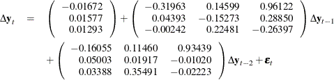
First, the differenced data is modeled as a VAR(2) with the following result:
The parameter estimates AR1_1_2, AR1_1_3, AR2_1_2, and AR2_1_3 are insignificant, and the VARX model is fitted in the next step.
The detailed output is shown in Output 42.2.1 through Output 42.2.8.
Output 42.2.1 shows the descriptive statistics.
Output 42.2.1: Descriptive Statistics
| Analysis of German Economic Variables |
| Number of Observations | 75 |
|---|---|
| Number of Pairwise Missing | 0 |
| Observation(s) eliminated by differencing | 1 |
| Simple Summary Statistics | ||||||||
|---|---|---|---|---|---|---|---|---|
| Variable | Type | N | Mean | Standard Deviation |
Min | Max | Difference | Label |
| y1 | Dependent | 75 | 0.01811 | 0.04680 | -0.14018 | 0.19358 | 1 | logarithm of investment |
| y2 | Dependent | 75 | 0.02071 | 0.01208 | -0.02888 | 0.05023 | 1 | logarithm of income |
| y3 | Dependent | 75 | 0.01987 | 0.01040 | -0.01300 | 0.04483 | 1 | logarithm of consumption |
Output 42.2.2 shows that a VAR(2) model is fit to the data.
Output 42.2.2: Parameter Estimates
| Analysis of German Economic Variables |
| Type of Model | VAR(2) |
|---|---|
| Estimation Method | Least Squares Estimation |
| Constant | |
|---|---|
| Variable | Constant |
| y1 | -0.01672 |
| y2 | 0.01577 |
| y3 | 0.01293 |
| AR | ||||
|---|---|---|---|---|
| Lag | Variable | y1 | y2 | y3 |
| 1 | y1 | -0.31963 | 0.14599 | 0.96122 |
| y2 | 0.04393 | -0.15273 | 0.28850 | |
| y3 | -0.00242 | 0.22481 | -0.26397 | |
| 2 | y1 | -0.16055 | 0.11460 | 0.93439 |
| y2 | 0.05003 | 0.01917 | -0.01020 | |
| y3 | 0.03388 | 0.35491 | -0.02223 | |
Output 42.2.3 shows the parameter estimates and their significance.
Output 42.2.3: Parameter Estimates, Continued
| Schematic Representation | |||
|---|---|---|---|
| Variable/Lag | C | AR1 | AR2 |
| y1 | . | -.. | ... |
| y2 | + | ... | ... |
| y3 | + | .+. | .+. |
| + is > 2*std error, - is < -2*std error, . is between, * is N/A | |||
| Model Parameter Estimates | ||||||
|---|---|---|---|---|---|---|
| Equation | Parameter | Estimate | Standard Error |
t Value | Pr > |t| | Variable |
| y1 | CONST1 | -0.01672 | 0.01723 | -0.97 | 0.3352 | 1 |
| AR1_1_1 | -0.31963 | 0.12546 | -2.55 | 0.0132 | y1(t-1) | |
| AR1_1_2 | 0.14599 | 0.54567 | 0.27 | 0.7899 | y2(t-1) | |
| AR1_1_3 | 0.96122 | 0.66431 | 1.45 | 0.1526 | y3(t-1) | |
| AR2_1_1 | -0.16055 | 0.12491 | -1.29 | 0.2032 | y1(t-2) | |
| AR2_1_2 | 0.11460 | 0.53457 | 0.21 | 0.8309 | y2(t-2) | |
| AR2_1_3 | 0.93439 | 0.66510 | 1.40 | 0.1647 | y3(t-2) | |
| y2 | CONST2 | 0.01577 | 0.00437 | 3.60 | 0.0006 | 1 |
| AR1_2_1 | 0.04393 | 0.03186 | 1.38 | 0.1726 | y1(t-1) | |
| AR1_2_2 | -0.15273 | 0.13857 | -1.10 | 0.2744 | y2(t-1) | |
| AR1_2_3 | 0.28850 | 0.16870 | 1.71 | 0.0919 | y3(t-1) | |
| AR2_2_1 | 0.05003 | 0.03172 | 1.58 | 0.1195 | y1(t-2) | |
| AR2_2_2 | 0.01917 | 0.13575 | 0.14 | 0.8882 | y2(t-2) | |
| AR2_2_3 | -0.01020 | 0.16890 | -0.06 | 0.9520 | y3(t-2) | |
| y3 | CONST3 | 0.01293 | 0.00353 | 3.67 | 0.0005 | 1 |
| AR1_3_1 | -0.00242 | 0.02568 | -0.09 | 0.9251 | y1(t-1) | |
| AR1_3_2 | 0.22481 | 0.11168 | 2.01 | 0.0482 | y2(t-1) | |
| AR1_3_3 | -0.26397 | 0.13596 | -1.94 | 0.0565 | y3(t-1) | |
| AR2_3_1 | 0.03388 | 0.02556 | 1.33 | 0.1896 | y1(t-2) | |
| AR2_3_2 | 0.35491 | 0.10941 | 3.24 | 0.0019 | y2(t-2) | |
| AR2_3_3 | -0.02223 | 0.13612 | -0.16 | 0.8708 | y3(t-2) | |
Output 42.2.4 shows the innovation covariance matrix estimates, the various information criteria results, and the tests for white noise
residuals. The residuals are uncorrelated except at lag 3 for  variable.
Output 42.2.4: Diagnostic Checks
| Covariances of Innovations | |||
|---|---|---|---|
| Variable | y1 | y2 | y3 |
| y1 | 0.00213 | 0.00007 | 0.00012 |
| y2 | 0.00007 | 0.00014 | 0.00006 |
| y3 | 0.00012 | 0.00006 | 0.00009 |
| Information Criteria | |
|---|---|
| AICC | -1527.51 |
| HQC | -1536.46 |
| AIC | -1561.11 |
| SBC | -1499.27 |
| FPEC | 2.18E-11 |
| Cross Correlations of Residuals | ||||
|---|---|---|---|---|
| Lag | Variable | y1 | y2 | y3 |
| 0 | y1 | 1.00000 | 0.13242 | 0.28275 |
| y2 | 0.13242 | 1.00000 | 0.55526 | |
| y3 | 0.28275 | 0.55526 | 1.00000 | |
| 1 | y1 | 0.01461 | -0.00666 | -0.02394 |
| y2 | -0.01125 | -0.00167 | -0.04515 | |
| y3 | -0.00993 | -0.06780 | -0.09593 | |
| 2 | y1 | 0.07253 | -0.00226 | -0.01621 |
| y2 | -0.08096 | -0.01066 | -0.02047 | |
| y3 | -0.02660 | -0.01392 | -0.02263 | |
| 3 | y1 | 0.09915 | 0.04484 | 0.05243 |
| y2 | -0.00289 | 0.14059 | 0.25984 | |
| y3 | -0.03364 | 0.05374 | 0.05644 | |
| Schematic Representation of Cross Correlations of Residuals |
||||
|---|---|---|---|---|
| Variable/Lag | 0 | 1 | 2 | 3 |
| y1 | +.+ | ... | ... | ... |
| y2 | .++ | ... | ... | ..+ |
| y3 | +++ | ... | ... | ... |
| + is > 2*std error, - is < -2*std error, . is between | ||||
| Portmanteau Test for Cross Correlations of Residuals |
|||
|---|---|---|---|
| Up To Lag | DF | Chi-Square | Pr > ChiSq |
| 3 | 9 | 9.69 | 0.3766 |
Output 42.2.5 describes how well each univariate equation fits the data. The residuals are off from the normality, but have no AR effects.
The residuals for  variable have the ARCH effect.
Output 42.2.5: Diagnostic Checks Continued
| Univariate Model ANOVA Diagnostics | ||||
|---|---|---|---|---|
| Variable | R-Square | Standard Deviation |
F Value | Pr > F |
| y1 | 0.1286 | 0.04615 | 1.62 | 0.1547 |
| y2 | 0.1142 | 0.01172 | 1.42 | 0.2210 |
| y3 | 0.2513 | 0.00944 | 3.69 | 0.0032 |
| Univariate Model White Noise Diagnostics | |||||
|---|---|---|---|---|---|
| Variable | Durbin Watson |
Normality | ARCH | ||
| Chi-Square | Pr > ChiSq | F Value | Pr > F | ||
| y1 | 1.96269 | 10.22 | 0.0060 | 12.39 | 0.0008 |
| y2 | 1.98145 | 11.98 | 0.0025 | 0.38 | 0.5386 |
| y3 | 2.14583 | 34.25 | <.0001 | 0.10 | 0.7480 |
| Univariate Model AR Diagnostics | ||||||||
|---|---|---|---|---|---|---|---|---|
| Variable | AR1 | AR2 | AR3 | AR4 | ||||
| F Value | Pr > F | F Value | Pr > F | F Value | Pr > F | F Value | Pr > F | |
| y1 | 0.01 | 0.9029 | 0.19 | 0.8291 | 0.39 | 0.7624 | 1.39 | 0.2481 |
| y2 | 0.00 | 0.9883 | 0.00 | 0.9961 | 0.46 | 0.7097 | 0.34 | 0.8486 |
| y3 | 0.68 | 0.4129 | 0.38 | 0.6861 | 0.30 | 0.8245 | 0.21 | 0.9320 |
Output 42.2.6 is the output in a matrix format associated with the PRINT=(IMPULSE=) option for the impulse response function and standard
errors. The  variable in the first row is an impulse variable. The variable in the first column is a response variable. The numbers, 0.96122, 0.41555, –0.40789 at lag 1 to 3 are decreasing.
Output 42.2.6: Impulse Response Function
| Simple Impulse Response by Variable | ||||
|---|---|---|---|---|
| Variable Response\Impulse |
Lag | y1 | y2 | y3 |
| y1 | 1 | -0.31963 | 0.14599 | 0.96122 |
| STD | 0.12546 | 0.54567 | 0.66431 | |
| 2 | -0.05430 | 0.26174 | 0.41555 | |
| STD | 0.12919 | 0.54728 | 0.66311 | |
| 3 | 0.11904 | 0.35283 | -0.40789 | |
| STD | 0.08362 | 0.38489 | 0.47867 | |
| y2 | 1 | 0.04393 | -0.15273 | 0.28850 |
| STD | 0.03186 | 0.13857 | 0.16870 | |
| 2 | 0.02858 | 0.11377 | -0.08820 | |
| STD | 0.03184 | 0.13425 | 0.16250 | |
| 3 | -0.00884 | 0.07147 | 0.11977 | |
| STD | 0.01583 | 0.07914 | 0.09462 | |
| y3 | 1 | -0.00242 | 0.22481 | -0.26397 |
| STD | 0.02568 | 0.11168 | 0.13596 | |
| 2 | 0.04517 | 0.26088 | 0.10998 | |
| STD | 0.02563 | 0.10820 | 0.13101 | |
| 3 | -0.00055 | -0.09818 | 0.09096 | |
| STD | 0.01646 | 0.07823 | 0.10280 | |
The proportions of decomposition of the prediction error covariances of three variables are given in Output 42.2.7. If you see the variable in the first column, then the output explains that about 64.713% of the one-step-ahead prediction error covariances
of the variable  is accounted for by its own innovations, about 7.995% is accounted for by
  innovations, and about 27.292% is accounted for by
  innovations.
Output 42.2.7: Proportions of Prediction Error Covariance Decomposition
| Proportions of Prediction Error Covariances by Variable | ||||
|---|---|---|---|---|
| Variable | Lead | y1 | y2 | y3 |
| y1 | 1 | 1.00000 | 0.00000 | 0.00000 |
| 2 | 0.95996 | 0.01751 | 0.02253 | |
| 3 | 0.94565 | 0.02802 | 0.02633 | |
| 4 | 0.94079 | 0.02936 | 0.02985 | |
| 5 | 0.93846 | 0.03018 | 0.03136 | |
| 6 | 0.93831 | 0.03025 | 0.03145 | |
| y2 | 1 | 0.01754 | 0.98246 | 0.00000 |
| 2 | 0.06025 | 0.90747 | 0.03228 | |
| 3 | 0.06959 | 0.89576 | 0.03465 | |
| 4 | 0.06831 | 0.89232 | 0.03937 | |
| 5 | 0.06850 | 0.89212 | 0.03938 | |
| 6 | 0.06924 | 0.89141 | 0.03935 | |
| y3 | 1 | 0.07995 | 0.27292 | 0.64713 |
| 2 | 0.07725 | 0.27385 | 0.64890 | |
| 3 | 0.12973 | 0.33364 | 0.53663 | |
| 4 | 0.12870 | 0.33499 | 0.53631 | |
| 5 | 0.12859 | 0.33924 | 0.53217 | |
| 6 | 0.12852 | 0.33963 | 0.53185 | |
The table in Output 42.2.8 gives forecasts and their prediction error covariances.
Output 42.2.8: Forecasts
| Forecasts | ||||||
|---|---|---|---|---|---|---|
| Variable | Obs | Time | Forecast | Standard Error |
95% Confidence Limits | |
| y1 | 77 | 1979:1 | 6.54027 | 0.04615 | 6.44982 | 6.63072 |
| 78 | 1979:2 | 6.55105 | 0.05825 | 6.43688 | 6.66522 | |
| 79 | 1979:3 | 6.57217 | 0.06883 | 6.43725 | 6.70708 | |
| 80 | 1979:4 | 6.58452 | 0.08021 | 6.42732 | 6.74173 | |
| 81 | 1980:1 | 6.60193 | 0.09117 | 6.42324 | 6.78063 | |
| y2 | 77 | 1979:1 | 7.68473 | 0.01172 | 7.66176 | 7.70770 |
| 78 | 1979:2 | 7.70508 | 0.01691 | 7.67193 | 7.73822 | |
| 79 | 1979:3 | 7.72206 | 0.02156 | 7.67980 | 7.76431 | |
| 80 | 1979:4 | 7.74266 | 0.02615 | 7.69140 | 7.79392 | |
| 81 | 1980:1 | 7.76240 | 0.03005 | 7.70350 | 7.82130 | |
| y3 | 77 | 1979:1 | 7.54024 | 0.00944 | 7.52172 | 7.55875 |
| 78 | 1979:2 | 7.55489 | 0.01282 | 7.52977 | 7.58001 | |
| 79 | 1979:3 | 7.57472 | 0.01808 | 7.53928 | 7.61015 | |
| 80 | 1979:4 | 7.59344 | 0.02205 | 7.55022 | 7.63666 | |
| 81 | 1980:1 | 7.61232 | 0.02578 | 7.56179 | 7.66286 | |
Output 42.2.9 shows that you cannot reject Granger noncausality from  to using the 0.05 significance level.
Output 42.2.9: Granger Causality Tests
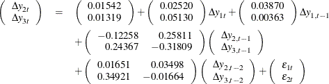
The following SAS statements show that the variable is the exogenous variable and fit the VARX(2,1) model to the data.
proc varmax data=use;
   id date interval=qtr;
   model y2 y3 = y1 / p=2 dify=(1) difx=(1) xlag=1 lagmax=3
                      print=(estimates diagnose);
run;
The fitted VARX(2,1) model is written as
The detailed output is shown in Output 42.2.10 through Output 42.2.13.
Output 42.2.10 shows the parameter estimates in terms of the constant, the current and the lag one coefficients of the exogenous variable, and the lag two coefficients of the dependent variables.
Output 42.2.10: Parameter Estimates
| Analysis of German Economic Variables |
| Type of Model | VARX(2,1) |
|---|---|
| Estimation Method | Least Squares Estimation |
| Constant | |
|---|---|
| Variable | Constant |
| y2 | 0.01542 |
| y3 | 0.01319 |
| XLag | ||
|---|---|---|
| Lag | Variable | y1 |
| 0 | y2 | 0.02520 |
| y3 | 0.05130 | |
| 1 | y2 | 0.03870 |
| y3 | 0.00363 | |
| AR | |||
|---|---|---|---|
| Lag | Variable | y2 | y3 |
| 1 | y2 | -0.12258 | 0.25811 |
| y3 | 0.24367 | -0.31809 | |
| 2 | y2 | 0.01651 | 0.03498 |
| y3 | 0.34921 | -0.01664 | |
Output 42.2.11 shows the parameter estimates and their significance.
Output 42.2.11: Parameter Estimates, Continued
| Model Parameter Estimates | ||||||
|---|---|---|---|---|---|---|
| Equation | Parameter | Estimate | Standard Error |
t Value | Pr > |t| | Variable |
| y2 | CONST1 | 0.01542 | 0.00443 | 3.48 | 0.0009 | 1 |
| XL0_1_1 | 0.02520 | 0.03130 | 0.81 | 0.4237 | y1(t) | |
| XL1_1_1 | 0.03870 | 0.03252 | 1.19 | 0.2383 | y1(t-1) | |
| AR1_1_1 | -0.12258 | 0.13903 | -0.88 | 0.3811 | y2(t-1) | |
| AR1_1_2 | 0.25811 | 0.17370 | 1.49 | 0.1421 | y3(t-1) | |
| AR2_1_1 | 0.01651 | 0.13766 | 0.12 | 0.9049 | y2(t-2) | |
| AR2_1_2 | 0.03498 | 0.16783 | 0.21 | 0.8356 | y3(t-2) | |
| y3 | CONST2 | 0.01319 | 0.00346 | 3.81 | 0.0003 | 1 |
| XL0_2_1 | 0.05130 | 0.02441 | 2.10 | 0.0394 | y1(t) | |
| XL1_2_1 | 0.00363 | 0.02536 | 0.14 | 0.8868 | y1(t-1) | |
| AR1_2_1 | 0.24367 | 0.10842 | 2.25 | 0.0280 | y2(t-1) | |
| AR1_2_2 | -0.31809 | 0.13546 | -2.35 | 0.0219 | y3(t-1) | |
| AR2_2_1 | 0.34921 | 0.10736 | 3.25 | 0.0018 | y2(t-2) | |
| AR2_2_2 | -0.01664 | 0.13088 | -0.13 | 0.8992 | y3(t-2) | |
Output 42.2.12 shows the innovation covariance matrix estimates, the various information criteria results, and the tests for white noise
residuals. The residuals is uncorrelated except at lag 3 for variable.
Output 42.2.12: Diagnostic Checks
| Covariances of Innovations | ||
|---|---|---|
| Variable | y2 | y3 |
| y2 | 0.00014 | 0.00006 |
| y3 | 0.00006 | 0.00009 |
| Information Criteria | |
|---|---|
| AICC | -1182.33 |
| HQC | -1177.94 |
| AIC | -1193.46 |
| SBC | -1154.52 |
| FPEC | 9.91E-9 |
| Cross Correlations of Residuals | |||
|---|---|---|---|
| Lag | Variable | y2 | y3 |
| 0 | y2 | 1.00000 | 0.56462 |
| y3 | 0.56462 | 1.00000 | |
| 1 | y2 | -0.02312 | -0.05927 |
| y3 | -0.07056 | -0.09145 | |
| 2 | y2 | -0.02849 | -0.05262 |
| y3 | -0.05804 | -0.08567 | |
| 3 | y2 | 0.16071 | 0.29588 |
| y3 | 0.10882 | 0.13002 | |
| Schematic Representation of Cross Correlations of Residuals |
||||
|---|---|---|---|---|
| Variable/Lag | 0 | 1 | 2 | 3 |
| y2 | ++ | .. | .. | .+ |
| y3 | ++ | .. | .. | .. |
| + is > 2*std error, - is < -2*std error, . is between | ||||
| Portmanteau Test for Cross Correlations of Residuals |
|||
|---|---|---|---|
| Up To Lag | DF | Chi-Square | Pr > ChiSq |
| 3 | 4 | 8.38 | 0.0787 |
Output 42.2.13 describes how well each univariate equation fits the data. The residuals are off from the normality, but have no ARCH and AR effects.
Output 42.2.13: Diagnostic Checks Continued
| Univariate Model ANOVA Diagnostics | ||||
|---|---|---|---|---|
| Variable | R-Square | Standard Deviation |
F Value | Pr > F |
| y2 | 0.0897 | 0.01188 | 1.08 | 0.3809 |
| y3 | 0.2796 | 0.00926 | 4.27 | 0.0011 |
| Univariate Model White Noise Diagnostics | |||||
|---|---|---|---|---|---|
| Variable | Durbin Watson |
Normality | ARCH | ||
| Chi-Square | Pr > ChiSq | F Value | Pr > F | ||
| y2 | 2.02413 | 14.54 | 0.0007 | 0.49 | 0.4842 |
| y3 | 2.13414 | 32.27 | <.0001 | 0.08 | 0.7782 |
| Univariate Model AR Diagnostics | ||||||||
|---|---|---|---|---|---|---|---|---|
| Variable | AR1 | AR2 | AR3 | AR4 | ||||
| F Value | Pr > F | F Value | Pr > F | F Value | Pr > F | F Value | Pr > F | |
| y2 | 0.04 | 0.8448 | 0.04 | 0.9570 | 0.62 | 0.6029 | 0.42 | 0.7914 |
| y3 | 0.62 | 0.4343 | 0.62 | 0.5383 | 0.72 | 0.5452 | 0.36 | 0.8379 |