SAMPLESIZE Statement :: SAS/STAT(R) 14.1 User's Guide

Option	Description
Fixed-Sample Models
INPUTNOBS	Specifies the sample size for a fixed-sample design
INPUTNEVENTS	Specifies the number of events for a fixed-sample design
One-Sample Models
ONESAMPLEMEAN	Specifies the one-sample Z test for the mean
ONESAMPLEFREQ	Specifies the one-sample test for the binomial proportion
Two-Sample Models
TWOSAMPLEMEAN	Specifies the two-sample Z test for the mean difference
TWOSAMPLEFREQ	Specifies the two-sample test for binomial proportions
TWOSAMPLESURVIVAL	Specifies the log-rank test for two survival distributions
Regression Models
REG	Specifies the test for a regression parameter
LOGISTIC	Specifies the test for a logistic regression parameter
PHREG	Specifies the test for a proportional hazards regression parameter

Fixed-Sample Models

The following two options compute the required sample size or number of events for a group sequential trial by using the sample size or number of events for the fixed-sample design:

MODEL=INPUTNOBS ( options )

specifies the input sample size from a fixed-sample study of nonsurvival data. The available options are as follows:

N=n
SAMPLE=ONE | TWO
WEIGHT= $w_ a$ < $w_ b$ >
MATCHNOBS=YES | NO

The required N=n option specifies the sample size n for the fixed-sample design. The SAMPLE=ONE option specifies a one-sample test, and the SAMPLE=TWO option specifies a two-sample test. The default is SAMPLE=ONE.

With a two-sample test, the WEIGHT= option specifies the sample size allocation weights for the two groups. If $w_{b}$ is not specified, $w_{b}= 1$ is used. The default is WEIGHT=1, which results in equal allocation for the two groups. The derived fractional sample sizes are rounded up to integers, and the MATCHNOBS=YES option requests these integer sample sizes to match the sample size allocation.

For more information about the input sample size for the fixed-sample design in sample size computation, see the section Input Sample Size for Fixed-Sample Design.

MODEL=INPUTNEVENTS ( D=d < options > )

specifies the number of events from a fixed-sample study of survival data. The required D=d option specifies the fixed-sample number of events d. To derive the sample size, you need to specify additional options from the following list:

ACCNOBS= $n_ a$
ACCRATE= $r_ a$
ACCRUAL=UNIFORM | EXP(PARM= $\gamma _0$ )
ACCTIME= $T_ a$
CEILING=TIME | N
FOLTIME= $T_ f$
HAZARD= $h_ a$ < $h_ b$ >
LOSS=NONE | EXP(HAZARD= $\tau$ | MEDLOSSTIME= $t_{\tau }$ )
MEDSURVTIME= $t_ a$ < $t_ b$ >
SAMPLE=ONE | TWO
TOTALTIME=T
WEIGHT= $w_ a$ < $w_ b$ >

The SAMPLE=ONE option specifies a one-sample test, and the SAMPLE=TWO option specifies a two-sample test. The default is SAMPLE=ONE. With a two-sample test, the WEIGHT= option specifies the sample size allocation weights for the two groups. If $w_ b$ is not specified, $w_ b$ =1 is used. The default is WEIGHT=1.

For a one-sample test, the HAZARD= $h_ a$ option specifies the hazard rate $h_ a$ explicitly, and the MEDSURVTIME= $t_ a$ option specifies the hazard rate implicitly through the median survival time $t_ a$ . Similarly, for a two-sample test, the HAZARD= $h_ a h_ b$ option specifies the hazard rates $h_ a$ and $h_ b$ for groups A and B explicitly, and the MEDSURVTIME= $t_ a t_ b$ option specifies hazard rates for groups A and B implicitly through the median survival times $t_ a$ and $t_ b$ . Also, for a two-sample test, $h_ b=h_ a$ if $h_ b$ is not specified and $t_ b=t_ a$ if $t_ b$ is not specified.

The ACCRUAL= option specifies the method for individual accrual. The ACCRUAL=UNIFORM option (which is the default) specifies that the individual accrual is uniform in the accrual time $T_ a$ with a constant accrual rate $r_ a$ , and the ACCRUAL=EXP(PARM= $\gamma _0$ ) option specifies that the individual accrual is truncated exponential with a scaled power parameter $\gamma _0$ , where $\gamma _0 \geq -10$ and $\gamma _0 \neq 0$ . With a scaled parameter $\gamma _0$ , the power parameter for the truncated exponential with the accrual time $T_ a$ is given by $\gamma = \gamma _0 / T_ a$ .

The ACCTIME= and FOLTIME= options specify the accrual time $T_ a$ and follow-up time $T_ f$ , respectively. The TOTALTIME= option specifies the total study time, $T= T_ a + T_ f$ .

The ACCRATE= option specifies the constant accrual rate $r_ a$ . If you specify the ACCRATE= option, then you must also specify one of the ACCTIME=, FOLTIME=, and TOTALTIME= options for the sample size computation. Otherwise, you must specify two of the ACCTIME=, FOLTIME=, and TOTALTIME= options to compute the accrual rate and sample size.

The ACCNOBS= option specifies the total number of individuals in the study. If you specify the ACCNOBS= option, then you must also specify one of the ACCTIME=, FOLTIME=, and TOTALTIME= options for the sample size computation. Otherwise, you must specify two of the ACCTIME=, FOLTIME=, and TOTALTIME= options to compute the accrual rate and sample size.

The CEILING= option specifies the additional sample size information to be displayed in the "Number of Events (D) and Sample Sizes (N)" table. The CEILING=TIME option (which is the default) displays additional information that includes ceiling times at the stages, and the CEILING=N option displays additional information that includes ceiling sample sizes at the stages. When you specify the SAMPLE=TWO option along with the CEILING=N option, the ceiling sample sizes at each stage are derived to match the sample size allocation weights for the two groups.

The LOSS= option specifies the individual loss to follow-up in the sample size computation. The LOSS=NONE option (which is the default) specifies no loss to follow-up, and the LOSS=EXP option specifies exponential loss function. The HAZARD= $\tau$ suboption specifies the exponential loss hazard rate $\tau$ , and the MEDLOSSTIME= $t_{\tau }$ suboption specifies the exponential loss hazard rate through the median loss times $t_{\tau }$ .

For a detailed description of the input number of events for the fixed-sample design in sample size computation, see the section Input Number of Events for Fixed-Sample Design.

One-Sample Models

The following two options compute the required sample size for a one-sample group sequential test:

MODEL=ONESAMPLEMEAN < ( options ) >

specifies the one-sample Z test for mean. The available options are as follows:

MEAN= $\mu _{1}$
STDDEV= $\sigma$

The MEAN= option specifies the alternative reference $\mu _{1}$ and is required if the alternative reference is not specified or derived in the procedure. If the MEAN=option is not specified, the specified or derived alternative reference is used.

The STDDEV= option specifies the standard deviation $\sigma$ . The default is STDDEV=1. See the section Test for a Normal Mean for a detailed description of the one-sample Z test for mean.

Note that the one-sample Z test for mean also includes the paired difference in two-treatment comparison (Jennison and Turnbull 2000, pp. 51–52), where $\mu _{1}$ is the mean of differences within pairs under the alternative hypothesis and $\sigma$ is the standard deviation for the mean of differences within pairs.

MODEL=ONESAMPLEFREQ < ( options ) >

specifies the one-sample test for binomial proportion with the null hypothesis $H_0: \theta = 0$ and the alternative hypothesis $H_1: \theta = \theta _1$ , where $\theta = p - p_0$ and $\theta _1= p_1 - p_0$ . The available options are as follows:

NULLPROP= $p_{0}$
PROP= $p_{1}$
REF= NULLPROP | PROP

The NULLPROP= and PROP= options specify the proportions under the null and alternative hypotheses, respectively. The default for the null reference is NULLPROP=0.5. The PROP= option is required if the alternative reference is not specified or derived in the procedure. If the PROP= option is not specified, the specified or derived alternative reference $\theta _1$ is used to compute the alternative reference $p_{1}= p_{0} + \theta _1$ .

The REF= option specifies the hypothesis under which the proportion is used in the sample size computation. The REF=NULLPROP option uses the null hypothesis, and the REF=PROP option uses the alternative hypothesis to compute the sample size. The default is REF=PROP. See the section Test for a Binomial Proportion for a detailed description of the one-sample tests for proportion.

Two-Sample Models

The following three options compute the required sample size or number of events for a two-sample group sequential trial.

MODEL=TWOSAMPLEMEAN < ( options ) >

specifies the two-sample Z test for mean difference. The available options are as follows:

MEANDIFF= $\theta _1$
STDDEV= $\sigma _{a} \, < \sigma _{b} >$
WEIGHT= $w_{a} \, < w_{b} >$
MATCHNOBS= YES | NO

The MEANDIFF= option specifies the alternative reference $\theta _1$ and is required if the alternative reference is not specified or derived in the procedure. If the MEANDIFF= option is not specified, the specified or derived alternative reference is used.

The STDDEV= option specifies the standard deviations $\sigma _{a}$ and $\sigma _{b}$ . If $\sigma _{b}$ is not specified, $\sigma _{b}= \sigma _{a}$ . The default is STDDEV=1.

The WEIGHT= option specifies the sample size allocation weights for the two groups. If $w_{b}$ is not specified, $w_{b}= 1$ is used. The default is WEIGHT=1, equal sample size for the two groups. The derived fractional sample sizes are rounded up to integers, and the MATCHNOBS=YES option requests these integer sample sizes to match the sample size allocation. The default is MATCHNOBS=NO.

See the section Test for the Difference between Two Normal Means for a detailed description of the two-sample Z test for mean difference.

MODEL=TWOSAMPLEFREQ < ( options ) >

specifies the two-sample test for binomial proportions. The available options are as follows:

NULLPROP= $p_{0a} < \, p_{0b} >$
PROP= $p_{1a}$
TEST= PROP | LOGOR | LOGRR
REF= NULLPROP | PROP | AVGNULLPROP | AVGPROP
WEIGHT= $w_{a} < \, w_{b} >$
MATCHNOBS= YES | NO

The NULLPROP= option specifies proportions $p_{a}= p_{0a}$ and $p_{b}= p_{0b}$ in groups A and B, respectively, under the null hypothesis. If $p_{0b}$ is not specified, $p_{0b}= p_{0a}$ . The default is NULLPROP=0.5.

The PROP= option specifies proportion $p_{a}= p_{1a}$ in group A under the alternative hypothesis. The proportion $p_{1b}$ in group B under the alternative hypothesis is given by $p_{1b}= p_{0b}$ . The PROP= option is required if the alternative reference is not specified or derived in the procedure. If the PROP= option is not specified, the specified or derived alternative reference is used to compute $p_{1a}$ , the proportion in group A under the alternative hypothesis.

The TEST= option specified the null hypothesis $H_{0}: \theta = 0$ in the test. The TEST=PROP option uses the difference in proportions $\theta = (p_{a} - p_{b}) - (p_{0a} - p_{0b})$ , the TEST=LOGOR option uses the log odds-ratio test $\theta = \delta - \delta _{0}$ , where

$\delta = \mr{log} \left( \frac{p_{a} (1-p_{b})}{p_{b} (1-p_{a})} \right) \, \, \, \, \, \, \, \, \delta _{0} = \mr{log} \left( \frac{p_{0a} (1-p_{0b})}{p_{0b} (1-p_{0a})} \right)$

and the TEST=LOGRR option uses the log relative risk test with $\theta = \delta - \delta _{0}$ , where

$\delta = \mr{log} \left( \frac{p_{a}}{p_{b}} \right) \, \, \, \, \, \, \, \, \delta _{0} = \mr{log} \left( \frac{p_{0a}}{p_{0b}} \right)$

The default is TEST=LOGOR.

The REF= option specifies the hypothesis under which the proportions are used in the sample size computation. The REF=NULLPROP option uses the null proportions $p_{0a}$ and $p_{0b}$ , the REF=PROP option uses the alternative proportions $p_{1a}$ and $p_{1b}$ , the REF=AVGNULLPROP option uses the average null proportion, and the REF=AVGPROP option uses the average alternative proportion. The default is REF=PROP.

The WEIGHT= option specifies the sample size allocation weights for the two groups. If $w_{b}$ is not specified, $w_{b}= 1$ is used. The default is WEIGHT=1, equal sample size for the two groups. The derived fractional sample sizes are also rounded up to integers, and the MATCHNOBS=YES option requests that these integer sample sizes match the sample size allocation.

See the section Test for the Difference between Two Binomial Proportions, the section Test for Two Binomial Proportions with a Log Odds Ratio Statistic, and the section Test for Two Binomial Proportions with a Log Relative Risk Statistic for a detailed description of the two-sample tests for proportions.

MODEL=TWOSAMPLESURVIVAL < ( options ) > MODEL=TWOSAMPLESURV < ( options ) >

specifies the log-rank test for two survival distributions with the null hypothesis 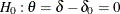$H_0: \theta = \delta - \delta _0= 0$ , where the parameter 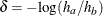$\delta = -\mr{log} (h_ a / h_ b)$ , $\delta _0$ is the value of $\delta$ under the null hypothesis and the values $h_ a$ and $h_ b$ are the constant hazard rates for groups A and B, respectively.

The available options for the number of events are as follows:

NULLHAZARD= $h_{0a} < \, h_{0b} >$
NULLMEDSURVTIME= $t_{0a} < \, t_{0b} >$
HAZARD= $h_{1a}$
HAZARDRATIO= $\lambda _{1}$
MEDSURVTIME= $t_{1a}$

The NULLHAZARD= option specifies hazard rates $h_{a}= h_{0a}$ and $h_{b}= h_{0b}$ for groups A and B, respectively, under the null hypothesis. If $h_{0b}$ is not specified, $h_{0b}= h_{0a}$ . The NULLMEDSURVTIME= option specifies the median survival times $t_{a}= t_{0a}$ and $t_{b}= t_{0b}$ under the null hypothesis. If $t_{0b}$ is not specified, $t_{0b}= t_{0a}$ . If both NULLHAZARD= and NULLMEDSURVTIME= option are not specified, NULLHAZARD=0.06931, which corresponds to NULLMEDSURVTIME=10, is used.

The hazard rate for group B under the alternative hypothesis, $h_{1b}$ , is identical to the hazard rate under the null hypothesis, $h_{0b}$ . The HAZARD=, MEDSURVTIME=, and HAZARDRATIO= options specify the group A hazard rate $h_{1a}$ , the group A median survival time $t_{1a}$ , and the hazard ratio $\lambda _{1}= h_{1a}/h_{1b}$ , respectively, under the alternative hypothesis. The HAZARD=, MEDSURVTIME=, or HAZARDRATIO= option is required if the alternative reference is not specified or derived in the procedure. If these three options are not specified, the specified or derived alternative reference $\theta _1$ is used to compute $h_{1a}$ from the equation:

$\theta _1= -\mr{log} \left( \frac{h_{1a}}{h_{1b}} \right) - \left( -\mr{log} \left( \frac{h_{0a}}{h_{0b}} \right) \right) = -\mr{log} \left( \frac{h_{1a}}{h_{0a}} \right)$

To derive the sample size, you need to specify additional options from the following list:

ACCNOBS= $n_ a$
ACCRATE= $r_ a$
ACCRUAL=UNIFORM | EXP(PARM= $\gamma _0$ )
ACCTIME= $T_ a$
CEILING=TIME | N
FOLTIME= $T_ f$
LOSS=NONE | EXP(HAZARD= $\tau$ | MEDLOSSTIME= $t_{\tau }$ )
REF=NULLHAZARD | HAZARD
TOTALTIME=T
WEIGHT= $w_ a$ < $w_ b$ >

The REF= option specifies the hypothesis under which the hazard is used in the sample size computation. The REF=NULLHAZARD option uses the null hypothesis, and the REF=HAZARD option uses the alternative hypothesis. The default is REF=HAZARD.

The WEIGHT= option specifies the sample size allocation weights for the two groups. If $w_{b}$ is not specified, $w_{b}= 1$ is used. The default is WEIGHT=1, equal sample size for the two groups.

The ACCRUAL= option specifies the method for individual accrual. The ACCRUAL=UNIFORM option (which is the default) specifies that the individual accrual is uniform in the accrual time $T_ a$ with a constant accrual rate $r_ a$ , and the ACCRUAL=EXP(PARM= $\gamma _0$ ) option specifies that the individual accrual is truncated exponential with a scaled power parameter $\gamma _0$ , where $\gamma _0 \geq -10$ and $\gamma _0 \neq 0$ . With a scaled parameter $\gamma _0$ , the power parameter for the truncated exponential with the accrual time $T_ a$ is given by $\gamma = \gamma _0 / T_ a$ .

The ACCTIME= and FOLTIME= options specify the accrual time $T_ a$ and follow-up time $T_ f$ , respectively. The TOTALTIME= option specifies the total study time, $T= T_ a + T_ f$ .

The ACCRATE= option specifies the constant accrual rate $r_ a$ . If you specify the ACCRATE= option, then you must also specify one of the ACCTIME=, FOLTIME=, and TOTALTIME= options for the sample size computation. Otherwise, you must specify two of the ACCTIME=, FOLTIME=, and TOTALTIME= options to compute the accrual rate and sample size.

The ACCNOBS= option specifies the total number of individuals in the study. If you specify the ACCNOBS= option, then you must also specify one of the ACCTIME=, FOLTIME=, and TOTALTIME= options for the sample size computation. Otherwise, you must specify two of the ACCTIME=, FOLTIME=, and TOTALTIME= options to compute the accrual rate and sample size.

The CEILING= option specifies the additional sample size information to be displayed in the "Number of Events (D) and Sample Sizes (N)" table. The CEILING=TIME option (which is the default) displays additional information that includes ceiling times at the stages, and the CEILING=N option displays additional information that includes ceiling sample sizes at the stages. When you specify CEILING=N, the ceiling sample sizes at each stage are derived to match the sample size allocation weights for the two groups.

The LOSS= option specifies the individual loss to follow-up in the sample size computation. The LOSS=NONE option (which is the default) specifies no loss to follow-up, and the LOSS=EXP option specifies exponential loss function. The HAZARD= $\tau$ suboption specifies the exponential loss hazard rate $\tau$ , and the MEDLOSSTIME= $t_{\tau }$ suboption specifies the exponential loss hazard rate through the median loss times $t_{\tau }$ .

See the section Test for Two Survival Distributions with a Log-Rank Test for a detailed description of the two-sample log-rank test for survival data.

Regression Models

The following three options compute the required sample size or number of events for group sequential tests on a regression parameter.

MODEL=REG < ( options ) >

specifies the Z test for a normal regression parameter. The available options are as follows:

BETA= $\beta _{1}$
VARIANCE= $\sigma ^{2}_{y}$
XVARIANCE= $\sigma ^{2}_{x}$
XRSQUARE= $r^{2}_{x}$

The BETA= option specifies the alternative reference $\beta _{1}$ and is required if the alternative reference is not specified or derived in the procedure. If the BETA= option is not specified, $\beta _{1}=\theta _1$ , the specified or derived alternative reference.

The VARIANCE= and XVARIANCE= options specify the variances for the response variable Y and covariate X, respectively. The defaults are VARIANCE=1 and XVARIANCE=1. For a model with more than one covariate, the XRSQUARE= option can be used to derive the variance of X after adjusting for other covariates. The default is XRSQUARE=0.

See the section Test for a Parameter in the Regression Model for a detailed description of the Z test for the regression parameter.

MODEL=LOGISTIC < ( options ) >

specifies the Z test for a logistic regression parameter. The available options are as follows:

BETA= $\beta _{1}$
PROP= p
XVARIANCE= $\sigma ^{2}_{x}$
XRSQUARE= $r^{2}_{x}$

The BETA= option specifies the alternative reference $\beta _{1}$ and is required if the alternative reference is not specified or derived in the procedure. If the BETA= option is not specified, $\beta _{1}=\theta _1$ , the specified or derived alternative reference.

The PROP= option specifies the proportion of the binary response variable Y. The default is PROP=0.5. The XVARIANCE= option specifies the variance of the covariate X. The default is XVARIANCE=1. For a model with more than one covariate, the XRSQUARE= option can be used to derive the variance of X after adjusting for other covariates. The default is XRSQUARE=0.

See the section Test for a Parameter in the Logistic Regression Model for a detailed description of the Z test for the logistic regression parameter.

MODEL=PHREG < ( options ) >

specifies the Z test for a proportional hazards regression parameter. The available options for the number of events are as follows:

BETA= $\beta _{1}$
XVARIANCE= $\sigma ^{2}_{x}$
XRSQUARE= $r^{2}_{x}$

The BETA= option specifies the alternative reference $\beta _{1}$ and is required if the alternative reference is not specified or derived in the procedure. If the BETA= option is not specified, $\beta _{1}=\theta _1$ , the specified or derived alternative reference.

The XVARIANCE= option specifies the variance of the covariate X. The default is XVARIANCE=1. For a model with more than one covariate, the XRSQUARE= option can be used to derive the variance of X after adjusting for other covariates. The default is XRSQUARE=0.

To derive the sample size, you need to specify additional options from the following list:

ACCNOBS= $n_ a$
ACCRATE= $r_ a$
ACCRUAL=UNIFORM | EXP(PARM= $\gamma _0$ )
ACCTIME= $T_ a$
CEILING=TIME | N
FOLTIME= $T_ f$
HAZARD= $h_ a$
LOSS=NONE | EXP(HAZARD= $\tau$ | MEDLOSSTIME= $t_{\tau }$ )
MEDSURVTIME= $t_ a$
TOTALTIME=T

The hazard rate is required for the sample size computation. The HAZARD= $h_{a}$ option specifies the hazard rate $h_{a}$ explicitly, and the MEDSURVTIME= $t_{a}$ option specifies the hazard rate implicitly through the median survival time $t_{a}$ .

The ACCRUAL= option specifies the method for individual accrual. The ACCRUAL=UNIFORM option (which is the default) specifies that the individual accrual is uniform in the accrual time $T_ a$ with a constant accrual rate $r_ a$ , and the ACCRUAL=EXP(PARM= $\gamma _0$ ) option specifies that the individual accrual is truncated exponential with a scaled power parameter $\gamma _0$ , where $\gamma _0 \geq -10$ and $\gamma _0 \neq 0$ . With a scaled parameter $\gamma _0$ , the power parameter for the truncated exponential with the accrual time $T_ a$ is given by $\gamma = \gamma _0 / T_ a$ .

The ACCTIME= and FOLTIME= options specify the accrual time $T_ a$ and follow-up time $T_ f$ , respectively. The TOTALTIME= option specifies the total study time, $T= T_ a + T_ f$ .

The ACCRATE= option specifies the constant accrual rate $r_ a$ . If you specify the ACCRATE= option, then you must also specify one of the ACCTIME=, FOLTIME=, and TOTALTIME= options for the sample size computation. Otherwise, you must specify two of the ACCTIME=, FOLTIME=, and TOTALTIME= options to compute the accrual rate and sample size.

The ACCNOBS= option specifies the total number of individuals in the study. If you specify the ACCNOBS= option, then you must also specify one of the ACCTIME=, FOLTIME=, and TOTALTIME= options for the sample size computation. Otherwise, you must specify two of the ACCTIME=, FOLTIME=, and TOTALTIME= options to compute the accrual rate and sample size.

The CEILING= option specifies the additional sample size information to be displayed in the "Number of Events (D) and Sample Sizes (N)" table. The CEILING=TIME option (which is the default) displays additional information that includes ceiling times at the stages, and the CEILING=N option displays additional information that includes ceiling sample sizes at the stages.

The LOSS= option specifies the individual loss to follow-up in the sample size computation. The LOSS=NONE option (which is the default) specifies no loss to follow-up, and the LOSS=EXP option specifies exponential loss function. The HAZARD= $\tau$ suboption specifies the exponential loss hazard rate $\tau$ , and the MEDLOSSTIME= $t_{\tau }$ suboption specifies the exponential loss hazard rate through the median loss times $t_{\tau }$ .

For a detailed description of the Z test for the proportional hazards regression parameter, see the section Test for a Parameter in the Proportional Hazards Regression Model.

The SEQDESIGN Procedure