The SEQDESIGN Procedure
-
Overview

- Getting Started
-
Syntax
-
DetailsFixed-Sample Clinical TrialsOne-Sided Fixed-Sample Tests in Clinical TrialsTwo-Sided Fixed-Sample Tests in Clinical TrialsGroup Sequential MethodsStatistical Assumptions for Group Sequential DesignsBoundary ScalesBoundary VariablesType I and Type II ErrorsUnified Family MethodsHaybittle-Peto MethodWhitehead MethodsError Spending MethodsAcceptance (beta) BoundaryBoundary Adjustments for Overlapping Lower and Upper beta BoundariesSpecified and Derived ParametersApplicable Boundary KeysSample Size ComputationApplicable One-Sample Tests and Sample Size ComputationApplicable Two-Sample Tests and Sample Size ComputationApplicable Regression Parameter Tests and Sample Size ComputationAspects of Group Sequential DesignsSummary of Methods in Group Sequential DesignsTable OutputODS Table NamesGraphics OutputODS Graphics
-
ExamplesCreating Fixed-Sample DesignsCreating a One-Sided O’Brien-Fleming DesignCreating Two-Sided Pocock and O’Brien-Fleming DesignsGenerating Graphics Display for Sequential DesignsCreating Designs Using Haybittle-Peto MethodsCreating Designs with Various Stopping CriteriaCreating Whitehead’s Triangular DesignsCreating a One-Sided Error Spending DesignCreating Designs with Various Number of StagesCreating Two-Sided Error Spending Designs with and without Overlapping Lower and Upper beta BoundariesCreating a Two-Sided Asymmetric Error Spending Design with Early Stopping to Reject H0Creating a Two-Sided Asymmetric Error Spending Design with Early Stopping to Reject or Accept H0Creating a Design with a Nonbinding Beta BoundaryComputing Sample Size for Survival Data That Have Uniform AccrualComputing Sample Size for Survival Data with Truncated Exponential Accrual
- References
Fixed-Sample Clinical Trials
A clinical trial is a research study in consenting human beings to answer specific health questions. One type of trial is a treatment trial, which tests the effectiveness of an experimental treatment. An example is a planned experiment designed to assess the efficacy of a treatment in humans by comparing the outcomes in a group of patients who receive the test treatment with the outcomes in a comparable group of patients who receive a placebo control treatment, where patients in both groups are enrolled, treated, and followed over the same time period.
A clinical trial is conducted according to a plan called a protocol. The protocol provides detailed description of the study. For a fixed-sample trial, the study protocol contains detailed information such as the null hypothesis, the one-sided or two-sided test, and the Type I and II error probability levels. It also includes the test statistic and its associated critical values in the hypothesis testing.
Generally, the efficacy of a new treatment is demonstrated by testing a hypothesis  in a clinical trial, where
  is the parameter of interest. For example, to test whether a population mean
  is greater than a specified value
  ,
,  can be used with an alternative
  .
.
A one-sided test is a test of the hypothesis with either an upper (greater) or a lower (lesser) alternative, and a two-sided
test is a test of the hypothesis with a two-sided alternative. The drug industry often prefers to use a one-sided test to
demonstrate clinical superiority based on the argument that a study should not be run if the test drug would be worse (Chow,
Shao, and Wang 2003, p. 28). But in practice, two-sided tests are commonly performed in drug development (Senn 1997, p. 161). For a fixed Type I error probability  , the sample sizes required by one-sided and two-sided tests are different. See Senn (1997, pp. 161–167) for a detailed description of issues involving one-sided and two-sided tests.
For independent and identically distributed observations  of a random variable, the likelihood function for is
![\[ L(\theta ) = \prod _{j=1}^{n} L_{i} (\theta ) \]](images/statug_seqdesign0184.png)
where is the population parameter and  is the probability or probability density of
  . Using the likelihood function, two statistics can be derived that are useful for inference: the maximum likelihood estimator
and the score statistic.
. Using the likelihood function, two statistics can be derived that are useful for inference: the maximum likelihood estimator
and the score statistic.
Maximum Likelihood Estimator
The maximum likelihood estimate (MLE)
of is the value  that maximizes the likelihood function for . Under mild regularity conditions, is an asymptotically unbiased estimate of with variance
  , where
  is the Fisher information
![\[ I(\theta ) = - \frac{ {\partial }^{2} \mr{log}( L(\theta ))}{\partial {\theta }^{2}} \]](images/statug_seqdesign0189.png)
and  is the expected Fisher information (Diggle et al. 2002, p. 340)
![\[ E_{\theta }( I(\theta ) ) = - E_{\theta } \left( \frac{ {\partial }^{2} \mr{log}( L(\theta ))}{\partial {\theta }^{2}} \right) \]](images/statug_seqdesign0191.png)
The score function for is defined as
![\[ S( \theta ) = \frac{ \partial \, \mr{log}( L(\theta )) }{\partial \theta } \]](images/statug_seqdesign0192.png)
and usually, the MLE can be derived by solving the likelihood equation  . Asymptotically, the MLE is normally distributed (Lindgren 1976, p. 272):
![\[ \hat{\theta } \sim N \left( \, \theta , \, \frac{1}{E_{\theta }( I(\theta ) )} \right) \]](images/statug_seqdesign0194.png)
If the Fisher information does not depend on , then is known. Otherwise, either the expected information evaluated at the MLE  (
( )
or the observed information
)
or the observed information  can be used for the Fisher information (Cox and Hinkley 1974, p. 302; Efron and Hinkley 1978, p. 458), where the observed Fisher information
![\[ I({\hat{\theta }}) = - \left( \frac{ {\partial }^{2} \mr{log}( L(\theta )) }{ \partial {\theta }^{2} } \, | \, \theta ={\hat\theta } \right) \]](images/statug_seqdesign0197.png)
If the Fisher information does depend on , the observed Fisher information is recommended for the variance of the maximum likelihood estimator (Efron and Hinkley 1978, p. 457).
Thus, asymptotically, for large n,
![\[ \hat{\theta } \sim N \left( \, \theta , \, \frac{1}{I} \right) \]](images/statug_seqdesign0198.png)
where I is the information, either the expected Fisher information  or the observed Fisher information
  .
.
So to test versus  , you can use the standardized Z test statistic
![\[ Z = \frac{\hat\theta }{\sqrt {\mr{Var}({\hat\theta })}} = {\hat\theta } \, \sqrt {I} \sim N \left( \, 0, \, 1 \right) \]](images/statug_seqdesign0201.png)
and the two-sided p-value is given by
![\[ \mr{Prob} (|Z| > |z_0|) = 1 - 2 \Phi (|z_0|) \]](images/statug_seqdesign0202.png)
where  is the cumulative standard normal distribution function and
  is the observed Z statistic.
If the BOUNDARYSCALE=SCORE is specified in the SEQDESIGN procedure, the boundary values for the test statistic are displayed
in the score statistic scale. With the standardized Z statistic, the score statistic  and
and
![\[ S \sim N \left( \, 0, \, I \right) \]](images/statug_seqdesign0205.png)
Score Statistic
The score statistic is based on the score function for ,
Under the null hypothesis , the score statistic  is the first derivative of the log likelihood evaluated at the null reference 0:
![\[ S(0) = \frac{ \partial \, \mr{log}( L(\theta )) }{\partial \theta } \, | \, \theta =0 \]](images/statug_seqdesign0207.png)
Under regularity conditions, is asymptotically normally distributed with mean zero and variance , the expected Fisher information evaluated at the null hypothesis  (Kalbfleisch and Prentice 1980, p. 45), where is the Fisher information
![\[ I(\theta ) = - E \left( \frac{ {\partial }^{2} \, \mr{log}( L(\theta )) }{ \partial {\theta }^{2} } \right) \]](images/statug_seqdesign0209.png)
That is, for large n,
![\[ S(0) \sim N \left( \, 0, \, E_{\theta =0} (I(\theta )) \right) \]](images/statug_seqdesign0210.png)
Asymptotically, the variance of the score statistic , , can also be replaced by the expected Fisher information evaluated at the MLE  (),
the observed Fisher information evaluated at the null hypothesis (
(),
the observed Fisher information evaluated at the null hypothesis ( ,
or the observed Fisher information evaluated at the MLE (
,
or the observed Fisher information evaluated at the MLE ( ) (Kalbfleisch and Prentice 1980, p. 46), where
![\[ I(0) = - \left( \frac{ {\partial }^{2} \mr{log}( L(\theta )) }{ \partial {\theta }^{2} } \, | \, \theta =0 \right) \]](images/statug_seqdesign0214.png)
Thus, asymptotically, for large n,
![\[ S(0) \sim N \left( \, 0, \, I \right) \]](images/statug_seqdesign0215.png)
where I is the information, either an expected Fisher information ( or ) or a observed Fisher information ( or ).
or ).
So to test versus , you can use the standardized Z test statistic
![\[ Z = \frac{S(0)}{\sqrt {I}} \]](images/statug_seqdesign0217.png)
If the BOUNDARYSCALE=MLE is specified in the SEQDESIGN procedure, the boundary values for the test statistic are displayed
in the MLE scale. With the standardized Z statistic, the MLE statistic 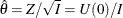 and
and
![\[ {\hat\theta } \sim N \left( \, 0, \, \frac{1}{I} \right) \]](images/statug_seqdesign0219.png)
One-Sample Test for Mean
The following one-sample test for mean is used to demonstrate fixed-sample clinical trials in the section One-Sided Fixed-Sample Tests in Clinical Trials and the section Two-Sided Fixed-Sample Tests in Clinical Trials.
Suppose  are n observations of a response variable
 Y from a normal distribution
![\[ y_{i} \sim N \left( \, \theta , \, {\sigma }^{2} \right) \]](images/statug_seqdesign0221.png)
where is the unknown mean and  is the known variance.
Then the log likelihood function for is
![\[ \mr{log} (L(\theta )) = \sum _{j=1}^{n} -\frac{1}{2} \frac{{(y_ j-\theta )}^{2}}{\sigma ^{2}} + c \]](images/statug_seqdesign0222.png)
where c is a constant. The first derivative is
![\[ \frac{ {\partial } \mr{log}( L(\theta )) }{ \partial {\theta } } = \frac{1}{\sigma ^{2}} \sum _{j=1}^{n} (y_ j - \theta ) = \frac{n}{\sigma ^{2}} ( {\overline{y}} - \theta ) \]](images/statug_seqdesign0223.png)
where  is the sample mean.
Setting the first derivative to zero, the MLE of is  , the sample mean. The variance for can be derived from the Fisher information
![\[ I(\theta ) = - \frac{ {\partial }^{2} \mr{log}( L(\theta )) }{ \partial {\theta }^{2} } = \frac{n}{\sigma ^{2}} \]](images/statug_seqdesign0226.png)
Since the Fisher information  does not depend on in this case,
  is used as the variance for . Thus the sample mean has a normal distribution with mean and variance
  :
:
![\[ \hat{\theta } = {\overline{y}} \sim N \left( \, \theta , \, \frac{1}{I_{0}} \right) = N \left( \, \theta , \, \frac{{\sigma }^{2}}{n} \right) \]](images/statug_seqdesign0230.png)
Under the null hypothesis , the score statistic
![\[ S(0) = \frac{ \partial \, \mr{log}( L(\theta )) }{\partial \theta } | \theta =0 = \frac{n}{\sigma ^{2}} {\overline{y}} \]](images/statug_seqdesign0231.png)
has a mean zero and variance
With the MLE , the corresponding standardized statistic is computed as 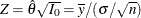 , which has a normal distribution with variance 1:
![\[ Z \sim N \left( \, {\theta } \sqrt {I_{0}}, \, 1 \right) = N \left( \, \frac{\theta }{\sigma / \sqrt {n}}, \, 1 \right) \]](images/statug_seqdesign0233.png)
Also, the corresponding score statistic is computed as 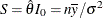 and
and
![\[ S \sim N \left( \, {\theta } I_{0}, \, I_{0} \right) = N \left( \, \frac{n \theta }{{\sigma }^{2}}, \, \frac{n}{{\sigma }^{2}} \right) \]](images/statug_seqdesign0235.png)
which is identical to computed under the null hypothesis .
Note that if the variable Y does not have a normal distribution, then it is assumed that the sample size n is large such that the sample mean has an approximately normal distribution.