The SEQDESIGN Procedure
-
Overview

- Getting Started
-
Syntax
-
DetailsFixed-Sample Clinical TrialsOne-Sided Fixed-Sample Tests in Clinical TrialsTwo-Sided Fixed-Sample Tests in Clinical TrialsGroup Sequential MethodsStatistical Assumptions for Group Sequential DesignsBoundary ScalesBoundary VariablesType I and Type II ErrorsUnified Family MethodsHaybittle-Peto MethodWhitehead MethodsError Spending MethodsAcceptance (beta) BoundaryBoundary Adjustments for Overlapping Lower and Upper beta BoundariesSpecified and Derived ParametersApplicable Boundary KeysSample Size ComputationApplicable One-Sample Tests and Sample Size ComputationApplicable Two-Sample Tests and Sample Size ComputationApplicable Regression Parameter Tests and Sample Size ComputationAspects of Group Sequential DesignsSummary of Methods in Group Sequential DesignsTable OutputODS Table NamesGraphics OutputODS Graphics
-
ExamplesCreating Fixed-Sample DesignsCreating a One-Sided O’Brien-Fleming DesignCreating Two-Sided Pocock and O’Brien-Fleming DesignsGenerating Graphics Display for Sequential DesignsCreating Designs Using Haybittle-Peto MethodsCreating Designs with Various Stopping CriteriaCreating Whitehead’s Triangular DesignsCreating a One-Sided Error Spending DesignCreating Designs with Various Number of StagesCreating Two-Sided Error Spending Designs with and without Overlapping Lower and Upper beta BoundariesCreating a Two-Sided Asymmetric Error Spending Design with Early Stopping to Reject H0Creating a Two-Sided Asymmetric Error Spending Design with Early Stopping to Reject or Accept H0Creating a Design with a Nonbinding Beta BoundaryComputing Sample Size for Survival Data That Have Uniform AccrualComputing Sample Size for Survival Data with Truncated Exponential Accrual
- References
Example 101.7 Creating Whitehead’s Triangular Designs
This example requests three 4-stage Whitehead’s triangular designs for normally distributed statistics. Each design has a
one-sided alternative hypothesis 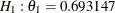 with early stopping to reject or accept the null hypothesis
  . Note that Whitehead’s triangular designs are different from unified family triangular designs.
The following statements invoke the SEQDESIGN procedure and specify three Whitehead’s triangular designs:
ods graphics on;
proc seqdesign altref=0.693147
               bscale=score
               plots=combinedboundary
               ;
   BoundaryKeyNone:  design nstages=4
                            method=whitehead
                            boundarykey=none
                            alt=upper   stop=both
                            alpha=0.05  beta=0.20
                            ;
   BoundaryKeyAlpha: design nstages=4
                            method=whitehead
                            boundarykey=alpha
                            alt=upper   stop=both
                            alpha=0.05  beta=0.20
                            ;

   BoundaryKeyBeta:  design nstages=4
                            method=whitehead
                            boundarykey=beta
                            alt=upper   stop=both
                            alpha=0.05  beta=0.20
                            ;
run;
Whitehead methods with early stopping to reject or accept the null hypothesis create boundaries that approximately satisfy the Type I and Type II error probability specification. The BOUNDARYKEY=NONE option specifies no adjustment to the boundary value at the final stage to maintain either a Type I or a Type II error probability level.
The "Design Information" table in Output 101.7.1 displays design specifications and maximum information. Note that with the BOUNDARYKEY=NONE option, the derived errors  and
and  are not the same as the specified errors
  and
and  .
.
Output 101.7.1: Whitehead Design Information
| Design Information | |
|---|---|
| Statistic Distribution | Normal |
| Boundary Scale | Score |
| Alternative Hypothesis | Upper |
| Early Stop | Accept/Reject Null |
| Method | Whitehead |
| Boundary Key | None |
| Alternative Reference | 0.693147 |
| Number of Stages | 4 |
| Alpha | 0.05071 |
| Beta | 0.19771 |
| Power | 0.80229 |
| Max Information (Percent of Fixed Sample) | 129.6815 |
| Max Information | 16.70639 |
| Null Ref ASN (Percent of Fixed Sample) | 62.48184 |
| Alt Ref ASN (Percent of Fixed Sample) | 73.82535 |
The "Method Information" table in Output 101.7.2 displays the derived  and
and  errors and the derived drift parameter. The derived errors and are not exactly the same as the specified errors and with the BOUNDARYKEY=NONE option.
Output 101.7.2: Method Information
The "Boundary Information" table in Output 101.7.3 displays information level, alternative reference, and boundary values. With the specified BOUNDARYSCALE=SCORE option, the alternative reference and boundary values are displayed with the score statistics scale.
Output 101.7.3: Boundary Information
| Boundary Information (Score Scale) Null Reference = 0 |
|||||
|---|---|---|---|---|---|
| _Stage_ | Alternative | Boundary Values | |||
| Information Level | Reference | Upper | |||
| Proportion | Actual | Upper | Beta | Alpha | |
| 1 | 0.2500 | 4.176597 | 2.89500 | -0.95755 | 4.78775 |
| 2 | 0.5000 | 8.353195 | 5.78999 | 1.91510 | 5.74530 |
| 3 | 0.7500 | 12.52979 | 8.68499 | 4.78775 | 6.70285 |
| 4 | 1.0000 | 16.70639 | 11.57998 | 7.66039 | 7.66039 |
With ODS Graphics enabled, a detailed boundary plot with the rejection and acceptance regions is displayed, as shown in Output 101.7.4.
Output 101.7.4: Boundary Plot
The second design uses the BOUNDARYKEY=ALPHA option to adjust the boundary value at the final stage to maintain the Type I error probability level.
The "Design Information" table in Output 101.7.5 displays design specifications and the derived maximum information. Note that with the BOUNDARYKEY=ALPHA option, the specified
Type I error probability is maintained.
Output 101.7.5: Whitehead Design Information
| Design Information | |
|---|---|
| Statistic Distribution | Normal |
| Boundary Scale | Score |
| Alternative Hypothesis | Upper |
| Early Stop | Accept/Reject Null |
| Method | Whitehead |
| Boundary Key | Alpha |
| Alternative Reference | 0.693147 |
| Number of Stages | 4 |
| Alpha | 0.05 |
| Beta | 0.20044 |
| Power | 0.79956 |
| Max Information (Percent of Fixed Sample) | 129.9894 |
| Max Information | 16.70639 |
| Null Ref ASN (Percent of Fixed Sample) | 62.6302 |
| Alt Ref ASN (Percent of Fixed Sample) | 74.00064 |
The "Method Information" table in Output 101.7.6 displays the specified and derived and errors and the derived drift parameter. The derived Type I error probability is the same as the specified and the derived Type II error probability  is not the same as the specified with the BOUNDARYKEY=ALPHA option.
Output 101.7.6: Method Information
The "Boundary Information" table in Output 101.7.7 displays information level, alternative reference, and boundary values.
Output 101.7.7: Boundary Information
| Boundary Information (Score Scale) Null Reference = 0 |
|||||
|---|---|---|---|---|---|
| _Stage_ | Alternative | Boundary Values | |||
| Information Level | Reference | Upper | |||
| Proportion | Actual | Upper | Beta | Alpha | |
| 1 | 0.2500 | 4.176597 | 2.89500 | -0.95755 | 4.78775 |
| 2 | 0.5000 | 8.353195 | 5.78999 | 1.91510 | 5.74530 |
| 3 | 0.7500 | 12.52979 | 8.68499 | 4.78775 | 6.70285 |
| 4 | 1.0000 | 16.70639 | 11.57998 | 7.81300 | 7.81300 |
With ODS Graphics enabled, a detailed boundary plot with the rejection and acceptance regions is displayed, as shown in Output 101.7.8.
Output 101.7.8: Boundary Plot

The third design specifies the BOUNDARYKEY=BETA option to derive the boundary values to maintain the Type II error probability
level .
The "Design Information" table in Output 101.7.9 displays design specifications and the derived maximum information. Note that with the BOUNDARYKEY=BETA option, the specified
Type II error probability is maintained.
Output 101.7.9: Whitehead Design Information
| Design Information | |
|---|---|
| Statistic Distribution | Normal |
| Boundary Scale | Score |
| Alternative Hypothesis | Upper |
| Early Stop | Accept/Reject Null |
| Method | Whitehead |
| Boundary Key | Beta |
| Alternative Reference | 0.693147 |
| Number of Stages | 4 |
| Alpha | 0.05011 |
| Beta | 0.2 |
| Power | 0.8 |
| Max Information (Percent of Fixed Sample) | 129.9364 |
| Max Information | 16.70639 |
| Null Ref ASN (Percent of Fixed Sample) | 62.60462 |
| Alt Ref ASN (Percent of Fixed Sample) | 73.97042 |
The "Method Information" table in Output 101.7.10 displays the and errors and the derived drift parameter. The derived Type II error probability is the same as the specified and the derived Type I error probability  is not the same as the specified with the BOUNDARYKEY=BETA option.
Output 101.7.10: Method Information
The "Boundary Information" table in Output 101.7.11 displays information level, alternative reference, and boundary values.
Output 101.7.11: Boundary Information
| Boundary Information (Score Scale) Null Reference = 0 |
|||||
|---|---|---|---|---|---|
| _Stage_ | Alternative | Boundary Values | |||
| Information Level | Reference | Upper | |||
| Proportion | Actual | Upper | Beta | Alpha | |
| 1 | 0.2500 | 4.176597 | 2.89500 | -0.95755 | 4.78775 |
| 2 | 0.5000 | 8.353195 | 5.78999 | 1.91510 | 5.74530 |
| 3 | 0.7500 | 12.52979 | 8.68499 | 4.78775 | 6.70285 |
| 4 | 1.0000 | 16.70639 | 11.57998 | 7.78899 | 7.78899 |
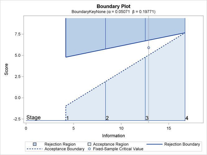
With ODS Graphics enabled, a detailed boundary plot with the rejection and acceptance regions is displayed, as shown in Output 101.7.12.
Output 101.7.12: Boundary Plot
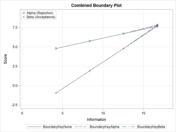
With the PLOTS=COMBINEDBOUNDARY option, a combined plot of group sequential boundaries for all designs is displayed, as shown in Output 101.7.13. It shows that three designs are similar, with a slightly smaller boundary value at the final stage for the design with the BOUNDARYKEY=NONE option.
Output 101.7.13: Combined Boundary Plot