The SEQDESIGN Procedure

For each sequential design, the and errors spent at each stage can be computed from the boundary values. For example, for a -stage design with an upper alternative hypothesis and early stopping to reject the null hypothesis , the boundary values in a standardized scale are the upper critical values , . At each interim stage, the null hypothesis is rejected if the observed standardized statistic . Otherwise, the process continues to the next stage. At the final stage, the hypothesis is rejected if . Otherwise, the null hypothesis is accepted.

The boundary values are derived such that the overall Type I error probability

where is the spending at stage . That is, at stage ,

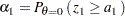At a subsequent stage ,

Since each design can be uniquely identified by the and errors spent at each stage, a design can then be derived by specifying the and errors to be used at each stage. The error spending method (Lan and DeMets 1983) distributes the error to be used at each stage and then derives the boundary values. Numerous forms of the error spending function are available. Kim and DeMets (1987) examine the functions , , and , where is the information fraction. Jennison and Turnbull (2000, p. 148) generalize these functions to the power functions .

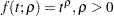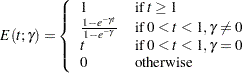
The ERRFUNCPOC option uses the cumulative error spending function (Lan and DeMets 1983)

With a specified error of or , the cumulative error spending at stage is or , where is the information fraction at stage . The method produces boundaries similar to those produced with Pocock’s method.

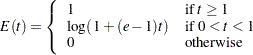
The ERRFUNCOBF option uses the cumulative error spending function (Lan and DeMets 1983)

where is either for the spending function or for the spending function. That is, with a specified error of or , the cumulative error spending at stage is or . The method produces boundaries similar to those produced with the O’Brien-Fleming method.

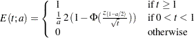
The ERRFUNCGAMMA option uses the gamma cumulative error spending function (Hwang, Shih, and DeCani 1990)

where is the parameter specified in the GAMMA= option. That is, with a specified error of or , the cumulative error spending at stage is or .

The ERRFUNCPOW option uses the cumulative error spending function (Jennison and Turnbull 2000, p. 148)

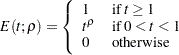where is the power parameter specified in the RHO= option. That is, with a specified error of or , the cumulative error spending at stage is or .

Error spending methods derive boundary values at each stage sequentially and require much more computation than other types of methods for group sequential trials with a large number of stages, especially for a two-sided asymmetric design with early stopping to accept , or to reject or accept .

Note that for a two-sided design with the STOP=BOTH or STOP=ACCEPT option, at each interim stage, the SEQDESIGN procedure first produces the lower and upper boundary values based on the one-sided spending. If the lower boundary value is greater than or equal to its corresponding upper boundary value, there is no early stopping to accept the null hypothesis at this stage, and the corresponding spending is distributed proportionally to the remaining stages.

For the error spending functions not available in the SEQDESIGN procedure, you can first compute the corresponding error spending at each stage explicitly, then use the SEQDESIGN procedure with the ERRSPEND= option to specify these errors directly.

For example, if the information levels are equally spaced in a five-stage design, the option ERRFUNCPOW (RHO=2) produces relative cumulative errors of , , , , and 1. This is equivalent to using the option ERRSPEND (1 4 9 16 25).

A one-sided error spending design is illustrated in Example 80.8 and a two-sided asymmetric error spending design is illustrated in Example 80.11.