The GENMOD Procedure

Poisson Regression

You can use the GENMOD procedure to fit a variety of statistical models. A typical use of PROC GENMOD is to perform Poisson regression.

You can use the Poisson distribution to model the distribution of cell counts in a multiway contingency table. Aitkin et al. (1989) have used this method to model insurance claims data. Suppose the following hypothetical insurance claims data are classified by two factors: age group (with two levels) and car type (with three levels).

data insure;
   input n c car$ age;
   ln = log(n);
   datalines;
500   42  small  1
1200  37  medium 1
100    1  large  1
400  101  small  2
500   73  medium 2
300   14  large  2
;

In the preceding data set, the variable n represents the number of insurance policyholders and the variable c represents the number of insurance claims. The variable car is the type of car involved (classified into three groups) and the variable age is the age group of a policyholder (classified into two groups).

You can use PROC GENMOD to perform a Poisson regression analysis of these data with a log link function. This type of model is sometimes called a log-linear model.

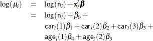
Assume that the number of claims c has a Poisson probability distribution and that its mean, $\mu _ i$ , is related to the factors car and age for observation i by

$\begin{eqnarray*} \log (\mu _ i) & = & \log ({\Variable{n}}_ i) + \mb{x}_ i^\prime \bbeta \\ & = & \log ({\Variable{n}}_ i) + \beta _{0} + \\ & & {\Variable{car}}_ i(1)\beta _{1} + {\Variable{car}}_ i(2)\beta _{2} + {\Variable{car}}_ i(3)\beta _{3} + \\ & & {\Variable{age}}_ i(1)\beta _{4} + {\Variable{age}}_ i(2)\beta _{5} \end{eqnarray*}$

The indicator variables $\mr{\Variable{car}}_ i(j)$ and $\mr{\Variable{age}}_ i(j)$ are associated with the jth level of the variables car and age for observation i

$\mr{\Variable{car}}_ i(j) = \left\{ \begin{array}{ll} 1 & \mr{if} \; \mr{\Variable{car}} = j \\ 0 & \mr{if} \; \mr{\Variable{car}} \neq j \end{array} \right.$

The $\beta$ s are unknown parameters to be estimated by the procedure. The logarithm of the variable n is used as an offset—that is, a regression variable with a constant coefficient of 1 for each observation. A log-linear relationship between the mean and the factors car and age is specified by the log link function. The log link function ensures that the mean number of insurance claims for each car and age group predicted from the fitted model is positive.

The following statements invoke the GENMOD procedure to perform this analysis:

proc genmod data=insure;
   class car age;
   model c = car age / dist   = poisson
                       link   = log
                       offset = ln;
run;

The variables car and age are specified as CLASS variables so that PROC GENMOD automatically generates the indicator variables associated with car and age.

The MODEL statement specifies c as the response variable and car and age as explanatory variables. An intercept term is included by default. Thus, the model matrix $\mb{X}$ (the matrix that has as its ith row the transpose of the covariate vector for the ith observation) consists of a column of 1s representing the intercept term and columns of 0s and 1s derived from indicator variables representing the levels of the car and age variables.

That is, the model matrix is

$\mb{X} = \left[ \begin{array}{r|rrr|rr} 1& 1& 0& 0& 1& 0 \\ 1& 0& 1& 0& 1& 0 \\ 1& 0& 0& 1& 1& 0 \\ 1& 1& 0& 0& 0& 1 \\ 1& 0& 1& 0& 0& 1 \\ 1& 0& 0& 1& 0& 1 \end{array} \right]$

where the first column corresponds to the intercept, the next three columns correspond to the variable car, and the last two columns correspond to the variable age.

The response distribution is specified as Poisson, and the link function is chosen to be log. That is, the Poisson mean parameter $\mu$ is related to the linear predictor by

$\log (\mu ) = \mb{x}_ i^\prime \bbeta$

The logarithm of n is specified as an offset variable, as is common in this type of analysis. In this case, the offset variable serves to normalize the fitted cell means to a per-policyholder basis, since the total number of claims, not individual policyholder claims, is observed. PROC GENMOD produces the following default output from the preceding statements.

Figure 44.1: Model Information

The GENMOD Procedure

Model Information
Data Set	WORK.INSURE
Distribution	Poisson
Link Function	Log
Dependent Variable	c
Offset Variable	ln

The "Model Information" table displayed in Figure 44.1 provides information about the specified model and the input data set.

Figure 44.2: Class Level Information

Class Level Information
Class	Levels	Values
car	3	large medium small
age	2	1 2

Figure 44.2 displays the "Class Level Information" table, which identifies the levels of the classification variables that are used in the model. Note that car is a character variable, and the values are sorted in alphabetical order. This is the default sort order, but you can select different sort orders with the ORDER= option in the PROC GENMOD statement.

Figure 44.3: Goodness of Fit

Criteria For Assessing Goodness Of Fit
Criterion	DF	Value	Value/DF
Deviance	2	2.8207	1.4103
Scaled Deviance	2	2.8207	1.4103
Pearson Chi-Square	2	2.8416	1.4208
Scaled Pearson X2	2	2.8416	1.4208
Log Likelihood		837.4533
Full Log Likelihood		-16.4638
AIC (smaller is better)		40.9276
AICC (smaller is better)		80.9276
BIC (smaller is better)		40.0946

The "Criteria For Assessing Goodness Of Fit" table displayed in Figure 44.3 contains statistics that summarize the fit of the specified model. These statistics are helpful in judging the adequacy of a model and in comparing it with other models under consideration. If you compare the deviance of 2.8207 with its asymptotic chi-square with 2 degrees of freedom distribution, you find that the p-value is 0.24. This indicates that the specified model fits the data reasonably well.

Figure 44.4: Analysis of Parameter Estimates

Analysis Of Maximum Likelihood Parameter Estimates
Parameter		DF	Estimate	Standard Error	Wald 95% Confidence Limits		Wald Chi-Square	Pr > ChiSq
Intercept		1	-1.3168	0.0903	-1.4937	-1.1398	212.73	<.0001
car	large	1	-1.7643	0.2724	-2.2981	-1.2304	41.96	<.0001
car	medium	1	-0.6928	0.1282	-0.9441	-0.4414	29.18	<.0001
car	small	0	0.0000	0.0000	0.0000	0.0000	.	.
age	1	1	-1.3199	0.1359	-1.5863	-1.0536	94.34	<.0001
age	2	0	0.0000	0.0000	0.0000	0.0000	.	.
Scale		0	1.0000	0.0000	1.0000	1.0000

Note:

The scale parameter was held fixed.

Figure 44.4 displays the "Analysis Of Parameter Estimates" table, which summarizes the results of the iterative parameter estimation process. For each parameter in the model, PROC GENMOD displays columns with the parameter name, the degrees of freedom associated with the parameter, the estimated parameter value, the standard error of the parameter estimate, the confidence intervals, and the Wald chi-square statistic and associated p-value for testing the significance of the parameter to the model. If a column of the model matrix corresponding to a parameter is found to be linearly dependent, or aliased, with columns corresponding to parameters preceding it in the model, PROC GENMOD assigns it zero degrees of freedom and displays a value of zero for both the parameter estimate and its standard error.

This table includes a row for a scale parameter, even though there is no free scale parameter in the Poisson distribution. See the section Response Probability Distributions for the form of the Poisson probability distribution. PROC GENMOD allows the specification of a scale parameter to fit overdispersed Poisson and binomial distributions. In such cases, the SCALE row indicates the value of the overdispersion scale parameter used in adjusting output statistics. See the section Overdispersion for more about overdispersion and the meaning of the SCALE parameter output by the GENMOD procedure. PROC GENMOD displays a note indicating that the scale parameter is fixed—that is, not estimated by the iterative fitting process.

It is usually of interest to assess the importance of the main effects in the model. Type 1 and Type 3 analyses generate statistical tests for the significance of these effects. You can request these analyses with the TYPE1 and TYPE3 options in the MODEL statement, as follows:

proc genmod data=insure;
   class car age;
   model c = car age / dist   = poisson
                       link   = log
                       offset = ln
                       type1
                       type3;
run;

The results of these analyses are summarized in the figures that follow.

Figure 44.5: Type 1 Analysis

The GENMOD Procedure

LR Statistics For Type 1 Analysis
Source	Deviance	DF	Chi-Square	Pr > ChiSq
Intercept	175.1536
car	107.4620	2	67.69	<.0001
age	2.8207	1	104.64	<.0001

In the table for Type 1 analysis displayed in Figure 44.5, each entry in the deviance column represents the deviance for the model containing the effect for that row and all effects preceding it in the table. For example, the deviance corresponding to car in the table is the deviance of the model containing an intercept and car. As more terms are included in the model, the deviance decreases.

Entries in the chi-square column are likelihood ratio statistics for testing the significance of the effect added to the model containing all the preceding effects. The chi-square value of 67.69 for car represents twice the difference in log likelihoods between fitting a model with only an intercept term and a model with an intercept and car. Since the scale parameter is set to 1 in this analysis, this is equal to the difference in deviances. Since two additional parameters are involved, this statistic can be compared with a chi-square distribution with two degrees of freedom. The resulting p-value (labeled Pr>Chi) of less than 0.0001 indicates that this variable is highly significant. Similarly, the chi-square value of 104.64 for age represents the difference in log likelihoods between the model with the intercept and car and the model with the intercept, car, and age. This effect is also highly significant, as indicated by the small p-value.

Figure 44.6: Type 3 Analysis

LR Statistics For Type 3 Analysis
Source	DF	Chi-Square	Pr > ChiSq
car	2	72.82	<.0001
age	1	104.64	<.0001

The Type 3 analysis results in the same conclusions as the Type 1 analysis. The Type 3 chi-square value for the car variable, for example, is twice the difference between the log likelihood for the model with the variables Intercept, car, and age included and the log likelihood for the model with the car variable excluded. The hypothesis tested in this case is the significance of the variable car given that the variable age is in the model. In other words, it tests the additional contribution of car in the model.

The values of the Type 3 likelihood ratio statistics for the car and age variables indicate that both of these factors are highly significant in determining the claims performance of the insurance policyholders.