The GENMOD Procedure
-
Overview

-
Getting Started
-
SyntaxPROC GENMOD StatementASSESS StatementBAYES StatementBY StatementCLASS StatementCODE StatementCONTRAST StatementDEVIANCE StatementEFFECTPLOT StatementESTIMATE StatementEXACT StatementEXACTOPTIONS StatementFREQ StatementFWDLINK StatementINVLINK StatementLSMEANS StatementLSMESTIMATE StatementMODEL StatementOUTPUT StatementProgramming StatementsREPEATED StatementSLICE StatementSTORE StatementSTRATA StatementVARIANCE StatementWEIGHT StatementZEROMODEL Statement
-
DetailsGeneralized Linear Models TheorySpecification of EffectsParameterization Used in PROC GENMODType 1 AnalysisType 3 AnalysisConfidence Intervals for ParametersF StatisticsLagrange Multiplier StatisticsPredicted Values of the MeanResidualsMultinomial ModelsZero-Inflated ModelsTweedie Distribution For Generalized Linear ModelsGeneralized Estimating EquationsAssessment of Models Based on Aggregates of ResidualsCase Deletion Diagnostic StatisticsBayesian AnalysisExact Logistic and Exact Poisson RegressionResponse Level OrderingMissing ValuesDisplayed Output for Classical AnalysisDisplayed Output for Bayesian AnalysisDisplayed Output for Exact AnalysisODS Table NamesODS Graphics
-
ExamplesLogistic RegressionNormal Regression, Log Link Gamma Distribution Applied to Life DataOrdinal Model for Multinomial DataGEE for Binary Data with Logit Link FunctionLog Odds Ratios and the ALR AlgorithmLog-Linear Model for Count DataModel Assessment of Multiple Regression Using Aggregates of ResidualsAssessment of a Marginal Model for Dependent DataBayesian Analysis of a Poisson Regression ModelExact Poisson RegressionTweedie Regression
- References
Exact Logistic and Exact Poisson Regression
The theory of exact logistic regression, also called exact conditional logistic regression, is described in the section Exact Conditional Logistic Regression in Chapter 72: The LOGISTIC Procedure. The following discussion of exact Poisson regression, also called exact conditional Poisson regression, uses the notation given in that section.
Note that in exact logistic regression, the coefficients  are the number of possible response vectors
  that generate
  :
:  . However, when performing an exact Poisson regression, this value is replaced by
![\[ C({\bm {t}}) = \sum _\Omega \prod _{i=1}^ n\frac{N_ i^{y_ i}}{y_ i!} \]](images/statug_genmod0634.png)
where 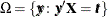 and
and  is the exponential of the offset
  for observation i. If an offset variable is not specified, then
  .
.
The probability density function (PDF) for  is created by summing over all candidate sequences that generate an observable
![\[ \Pr (\bT =\bm {t}) = \frac{C({\bm {t}})\exp ({\bm {t}}'\bbeta )}{\prod _{i=1}^ n\exp (N_ ie^{\bm {x}_ i'\bbeta })} \]](images/statug_genmod0639.png)
However, the conditional likelihood of  given
given  has the same form as that for exact logistic regression.
For details about hypothesis testing and estimation, see the sections Hypothesis Tests and Inference for a Single Parameter in Chapter 72: The LOGISTIC Procedure. See the section Computational Resources for Exact Logistic Regression in Chapter 72: The LOGISTIC Procedure, for some computational notes about exact analyses.
In exact logistic binary regression, each component  of can take a value of 0 or 1, so there are a finite number,
  , of candidate vectors to be considered. Since a Poisson-distributed response variable can take an infinite number of values, exact Poisson
regression should evaluate an infinite number of vectors. However, by identifying the maximum value of
, of candidate vectors to be considered. Since a Poisson-distributed response variable can take an infinite number of values, exact Poisson
regression should evaluate an infinite number of vectors. However, by identifying the maximum value of  to check,
  , for each observation i, the number of candidate vectors to check is reduced to
  . On a practical level, as becomes large the probability of the Poisson random variable achieving this value drops to zero, so can be thought of as the point at which the value does not matter. You can provide these maxima by specifying either an OFFSET=
variable, , or an EXACTMAX=
variable,
. On a practical level, as becomes large the probability of the Poisson random variable achieving this value drops to zero, so can be thought of as the point at which the value does not matter. You can provide these maxima by specifying either an OFFSET=
variable, , or an EXACTMAX=
variable,  , or you can let the algorithm choose a maximum for you. The way these two options interact to provide a maximum is described
in the following list:
, or you can let the algorithm choose a maximum for you. The way these two options interact to provide a maximum is described
in the following list:
-
If an EXACTMAX= variable is specified, then
 .
.
-
If the EXACTMAX option is specified without a variable, or if neither the EXACTMAX= nor OFFSET= options are specified, then you must also condition out the intercept or you must specify the STRATA statement. If you are conditioning out the intercept, then every
has an effective maximum of  , where
  is the observed response and
  is the frequency of the observation; this is the sufficient statistic for the intercept term. If you are performing a stratified
analysis, these sums are computed within each stratum.
is the frequency of the observation; this is the sufficient statistic for the intercept term. If you are performing a stratified
analysis, these sums are computed within each stratum.
-
If an offset variable is specified and the EXACTMAX option is not specified, then
 . For example, if you have
  rats in cage i and you are modeling the proportion that acquire a disease, then you would set your offsets to
  so that
  . In this case, the offsets must also satisfy
  .
.
OUTDIST= Output Data Set
The OUTDIST= data set contains every exact conditional distribution necessary to process the corresponding EXACT
statement. For example, the following statements create one distribution for the x1 parameter and another for the x2 parameters, and produce the data set dist shown in Table 44.11:
data test;
   input y x1 x2 count;
   datalines;
0 0 0 1
1 0 0 1
0 1 1 2
1 1 1 1
1 0 2 3
1 1 2 1
1 2 0 3
1 2 1 2
1 2 2 1
;
proc genmod data=test exactonly;
   class x2 / param=ref;
   model y=x1 x2 / d=b;
   exact x1 x2/ outdist=dist;
run;
proc print data=dist;
run;
Table 44.11: OUTDIST= Data Set
|
Obs |
x1 |
x20 |
x21 |
Count |
Score |
Prob |
|---|---|---|---|---|---|---|
|
1 |
. |
0 |
0 |
3 |
5.81151 |
0.03333 |
|
2 |
. |
0 |
1 |
15 |
1.66031 |
0.16667 |
|
3 |
. |
0 |
2 |
9 |
3.12728 |
0.10000 |
|
4 |
. |
1 |
0 |
15 |
1.46523 |
0.16667 |
|
5 |
. |
1 |
1 |
18 |
0.21675 |
0.20000 |
|
6 |
. |
1 |
2 |
6 |
4.58644 |
0.06667 |
|
7 |
. |
2 |
0 |
19 |
1.61869 |
0.21111 |
|
8 |
. |
2 |
1 |
2 |
3.27293 |
0.02222 |
|
9 |
. |
3 |
0 |
3 |
6.27189 |
0.03333 |
|
10 |
2 |
. |
. |
6 |
3.03030 |
0.12000 |
|
11 |
3 |
. |
. |
12 |
0.75758 |
0.24000 |
|
12 |
4 |
. |
. |
11 |
0.00000 |
0.22000 |
|
13 |
5 |
. |
. |
18 |
0.75758 |
0.36000 |
|
14 |
6 |
. |
. |
3 |
3.03030 |
0.06000 |
The first nine observations in the dist data set contain an exact distribution for the parameters of the x2 effect (hence the values for the x1 parameter are missing), and the remaining five observations are for the x1 parameter. If a joint distribution was created, there would be observations with values for both the x1 and x2 parameters. For CLASS
variables, the corresponding parameters in the dist data set are identified by concatenating the variable name with the appropriate classification level.
The data set contains the possible sufficient statistics of the parameters for the effects specified in the EXACT
statement, and the Count variable contains the number of different responses that yield these statistics. In particular, there are six possible response
vectors  for which the dot product
  was equal to 2, and for which
  ,
,  , and
, and  were equal to their actual observed values (displayed in the "Sufficient Statistics" table).
Note: If you are performing an exact Poisson analysis, then the Count variable is replaced by a variable named Weight.
When hypothesis tests are performed on the parameters, the Prob variable contains the probability of obtaining that statistic (which is just the count divided by the total count), and the
Score variable contains the score for that statistic.
The OUTDIST= data set can contain a different exact conditional distribution for each specified EXACT statement. For example, consider the following EXACT statements:
exact 'O1'   x1    /           outdist=o1;
exact 'OJ12' x1 x2 / jointonly outdist=oj12;
exact 'OA12' x1 x2 / joint     outdist=oa12;
exact 'OE12' x1 x2 / estimate  outdist=oe12;
The O1 statement outputs a single exact conditional distribution. The OJ12 statement outputs only the joint distribution for
x1 and x2. The OA12 statement outputs three conditional distributions: one for x1, one for x2, and one jointly for x1 and x2. The OE12 statement outputs two conditional distributions: one for x1 and the other for x2. Data set oe12 contains both the x1 and x2 variables; the distribution for x1 has missing values in the x2 column while the distribution for x2 has missing values in the x1 column.