The LOGISTIC Procedure

Exact Conditional Logistic Regression

The theory of exact logistic regression, also known as exact conditional logistic regression, was originally laid out by Cox (1970), and the computational methods employed in PROC LOGISTIC are described in Hirji, Mehta, and Patel (1987), Hirji (1992), and Mehta, Patel, and Senchaudhuri (1992). Other useful references for the derivations include Cox and Snell (1989), Agresti (1990), and Mehta and Patel (1995).

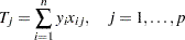
Exact conditional inference is based on generating the conditional distribution for the sufficient statistics of the parameters of interest. This distribution is called the permutation or exact conditional distribution. Using the notation in the section Computational Details, follow Mehta and Patel (1995) and first note that the sufficient statistics $\text{[math]}$ for the parameter vector of intercepts and slopes, $\text{[math]}$ , are

$\text{[math]}$

Denote a vector of observable sufficient statistics as $\text{[math]}$ .

The probability density function (pdf) for $\text{[math]}$ can be created by summing over all binary sequences $\text{[math]}$ that generate an observable $\text{[math]}$ and letting 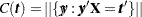$\text{[math]}$ denote the number of sequences $\text{[math]}$ that generate $\text{[math]}$

$\text{[math]}$

In order to condition out the nuisance parameters, partition the parameter vector $\text{[math]}$ , where $\text{[math]}$ is a $\text{[math]}$ vector of the nuisance parameters, and $\text{[math]}$ is the parameter vector for the remaining $\text{[math]}$ parameters of interest. Likewise, partition $\text{[math]}$ into $\text{[math]}$ and $\text{[math]}$ , $\text{[math]}$ into $\text{[math]}$ and $\text{[math]}$ , and $\text{[math]}$ into $\text{[math]}$ and $\text{[math]}$ . 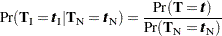The nuisance parameters can be removed from the analysis by conditioning on their sufficient statistics to create the conditional likelihood of $\text{[math]}$ given $\text{[math]}$ ,

	$\text{[math]}$	$\text{[math]}$	$\text{[math]}$
	$\text{[math]}$	$\text{[math]}$	$\text{[math]}$

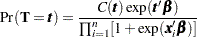
where $\text{[math]}$ is the number of vectors $\text{[math]}$ such that $\text{[math]}$ and $\text{[math]}$ . Note that the nuisance parameters have factored out of this equation, and that $\text{[math]}$ is a constant.

The goal of the exact conditional analysis is to determine how likely the observed response $\text{[math]}$ is with respect to all $\text{[math]}$ possible responses $\text{[math]}$ . One way to proceed is to generate every $\text{[math]}$ vector for which $\text{[math]}$ , and count the number of vectors $\text{[math]}$ for which $\text{[math]}$ is equal to each unique $\text{[math]}$ . Generating the conditional distribution from complete enumeration of the joint distribution is conceptually simple; however, this method becomes computationally infeasible very quickly. For example, if you had only $\text{[math]}$ observations, you would have to scan through $\text{[math]}$ different $\text{[math]}$ vectors.

Several algorithms are available in PROC LOGISTIC to generate the exact distribution. All of the algorithms are based on the following observation. Given any $\text{[math]}$ and a design $\text{[math]}$ , let $\text{[math]}$ and $\text{[math]}$ be the first $\text{[math]}$ rows of each matrix. Write the sufficient statistic based on these $\text{[math]}$ rows as $\text{[math]}$ . A recursion relation results: $\text{[math]}$ .

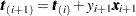The following methods are available:

The multivariate shift algorithm developed by Hirji, Mehta, and Patel (1987), which steps through the recursion relation by adding one observation at a time and building an intermediate distribution at each step. If it determines that $\text{[math]}$ for the nuisance parameters could eventually equal $\text{[math]}$ , then $\text{[math]}$ is added to the intermediate distribution.
An extension of the multivariate shift algorithm to generalized logit models by Hirji (1992). Since the generalized logit model fits a new set of parameters to each logit, the number of parameters in the model can easily get too large for this algorithm to handle. Note for these models that the hypothesis tests for each effect are computed across the logit functions, while individual parameters are estimated for each logit function.
A network algorithm described in Mehta, Patel, and Senchaudhuri (1992), which builds a network for each parameter that you are conditioning out in order to identify feasible $\text{[math]}$ for the $\text{[math]}$ vector. These networks are combined and the set of feasible $\text{[math]}$ is further reduced, and then the multivariate shift algorithm uses this knowledge to build the exact distribution without adding as many intermediate $\text{[math]}$ as the multivariate shift algorithm does.
A hybrid Monte Carlo and network algorithm described by Mehta, Patel, and Senchaudhuri (2000), which extends their 1992 algorithm by sampling from the combined network to build the exact distribution.

The bulk of the computation time and memory for these algorithms is consumed by the creation of the networks and the exact joint distribution. After the joint distribution for a set of effects is created, the computational effort required to produce hypothesis tests and parameter estimates for any subset of the effects is (relatively) trivial. See the section Computational Resources for Exact Logistic Regression for more computational notes about exact analyses.

Note: An alternative to using these exact conditional methods is to perform Firth’s bias-reducing penalized likelihood method (see the FIRTH option in the MODEL statement); this method has the advantage of being much faster and less memory intensive than exact algorithms, but it might not converge to a solution.

Hypothesis Tests

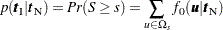
Consider testing the null hypothesis $\text{[math]}$ against the alternative $\text{[math]}$ , conditional on $\text{[math]}$ . Under the null hypothesis, the test statistic for the exact probability test is just $\text{[math]}$ , while the corresponding p-value is the probability of getting a less likely (more extreme) statistic,

$\text{[math]}$

where $\text{[math]}$ there exist $\text{[math]}$ with $\text{[math]}$ , $\text{[math]}$ , and $\text{[math]}$ .

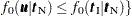For the exact conditional scores test, the conditional mean $\text{[math]}$ and variance matrix $\text{[math]}$ of the $\text{[math]}$ (conditional on $\text{[math]}$ ) are calculated, and the score statistic for the observed value,

$\text{[math]}$

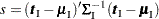is compared to the score for each member of the distribution

$\text{[math]}$

The resulting p-value is

$\text{[math]}$

where $\text{[math]}$ there exist $\text{[math]}$ with $\text{[math]}$ , $\text{[math]}$ , and $\text{[math]}$ .

The mid- $\text{[math]}$ statistic, defined as

$\text{[math]}$

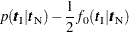was proposed by Lancaster (1961) to compensate for the discreteness of a distribution. See Agresti (1992) for more information. However, to allow for more flexibility in handling ties, you can write the mid- $\text{[math]}$ statistic as (based on a suggestion by Lamotte (2002) and generalizing Vollset, Hirji, and Afifi (1991))

$\text{[math]}$

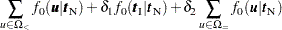where, for $\text{[math]}$ , $\text{[math]}$ is $\text{[math]}$ using strict inequalities, and $\text{[math]}$ is $\text{[math]}$ using equalities with the added restriction that $\text{[math]}$ . Letting $\text{[math]}$ yields Lancaster’s mid- $\text{[math]}$ .

Caution: When the exact distribution has ties and METHOD=NETWORKMC is specified, the Monte Carlo algorithm estimates $\text{[math]}$ with error, and hence it cannot determine precisely which values contribute to the reported p-values. For example, if the exact distribution has densities $\text{[math]}$ and if the observed statistic has probability $\text{[math]}$ , then the exact probability p-value is exactly $\text{[math]}$ . Under Monte Carlo sampling, if the densities after $\text{[math]}$ samples are $\text{[math]}$ and the observed probability is $\text{[math]}$ , then the resulting p-value is $\text{[math]}$ . Therefore, the exact probability test p-value for this example fluctuates between $\text{[math]}$ , $\text{[math]}$ , and $\text{[math]}$ , and the reported p-values are actually lower bounds for the true p-values. If you need more precise values, you can specify the OUTDIST= option, determine appropriate cutoff values for the observed probability and score, and then construct the true p-value estimates from the OUTDIST= data set and display them in the SAS log by using the following statements:

data _null_;
   set outdist end=end;
   retain pvalueProb 0 pvalueScore 0;
   if prob < ProbCutOff then pvalueProb+prob;
   if score > ScoreCutOff then pvalueScore+prob;
   if end then put pvalueProb= pvalueScore=;
run;

Inference for a Single Parameter

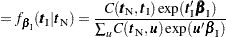
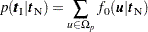
Exact parameter estimates are derived for a single parameter $\text{[math]}$ by regarding all the other parameters $\text{[math]}$ as nuisance parameters. The appropriate sufficient statistics are $\text{[math]}$ and $\text{[math]}$ , with their observed values denoted by the lowercase $\text{[math]}$ . Hence, the conditional pdf used to create the parameter estimate for $\text{[math]}$ is

$\text{[math]}$

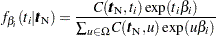for $\text{[math]}$ .

The maximum exact conditional likelihood estimate is the quantity $\text{[math]}$ , which maximizes the conditional pdf. A Newton-Raphson algorithm is used to perform this search. However, if the observed $\text{[math]}$ attains either its maximum or minimum value in the exact distribution (that is, either 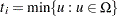$\text{[math]}$ or $\text{[math]}$ ), then the conditional pdf is monotonically increasing in $\text{[math]}$ and cannot be maximized. In this case, a median unbiased estimate (Hirji, Tsiatis, and Mehta; 1989) $\text{[math]}$ is produced that satisfies $\text{[math]}$ , and a Newton-Raphson algorithm is used to perform the search.

The standard error of the exact conditional likelihood estimate is just the negative of the inverse of the second derivative of the exact conditional log likelihood (Agresti; 2002).

Likelihood ratio tests based on the conditional pdf are used to test the null $\text{[math]}$ against the alternative $\text{[math]}$ . The critical region for this UMP test consists of the upper tail of values for $\text{[math]}$ in the exact distribution. Thus, the one-sided significance level $\text{[math]}$ is

$\text{[math]}$

Similarly, the one-sided significance level $\text{[math]}$ against $\text{[math]}$ is

$\text{[math]}$

The two-sided significance level $\text{[math]}$ against $\text{[math]}$ is calculated as

$\text{[math]}$

An upper $\text{[math]}$ % exact confidence limit for $\text{[math]}$ corresponding to the observed $\text{[math]}$ is the solution $\text{[math]}$ of $\text{[math]}$ , while the lower exact confidence limit is the solution $\text{[math]}$ of $\text{[math]}$ . Again, a Newton-Raphson procedure is used to search for the solutions. Note that one of the confidence limits for a median unbiased estimate is set to infinity, but the other is still computed at $\text{[math]}$ . This results in the display of a one-sided $\text{[math]}$ % confidence interval; if you want the $\text{[math]}$ limit instead, you can specify the ONESIDED option.

Specifying the ONESIDED option displays only one p-value and one confidence interval, because small values of $\text{[math]}$ and $\text{[math]}$ support different alternative hypotheses and only one of these p-values can be less than 0.50.

The mid-p confidence limits are the solutions to $\text{[math]}$ for $\text{[math]}$ (Vollset, Hirji, and Afifi; 1991). $\text{[math]}$ produces the usual exact (or max- $\text{[math]}$ ) confidence interval, $\text{[math]}$ yields the mid- $\text{[math]}$ interval, and $\text{[math]}$ gives the min- $\text{[math]}$ interval. The mean of the endpoints of the max- $\text{[math]}$ and min- $\text{[math]}$ intervals provides the mean- $\text{[math]}$ interval as defined by Hirji, Mehta, and Patel (1988).

Estimates and confidence intervals for the odds ratios are produced by exponentiating the estimates and interval endpoints for the parameters.

Notes about Exact p-Values

In the "Conditional Exact Tests" table, the exact probability test is not necessarily a sum of tail areas and can be inflated if the distribution is skewed. The more robust exact conditional scores test is a sum of tail areas and is generally preferred over the exact probability test.

The p-value reported for a single parameter in the "Exact Parameter Estimates" table is twice the one-sided tail area of a likelihood ratio test against the null hypothesis of the parameter equaling zero.