The LOGISTIC Procedure
- Overview
- Getting Started
-
Syntax
 PROC LOGISTIC Statement BY Statement CLASS Statement CONTRAST Statement EFFECT Statement EFFECTPLOT Statement ESTIMATE Statement EXACT Statement EXACTOPTIONS Statement FREQ Statement LSMEANS Statement LSMESTIMATE Statement MODEL Statement ODDSRATIO Statement OUTPUT Statement ROC Statement ROCCONTRAST Statement SCORE Statement SLICE Statement STORE Statement STRATA Statement TEST Statement UNITS Statement WEIGHT Statement
 -
Details
Missing Values Response Level Ordering Link Functions and the Corresponding Distributions Determining Observations for Likelihood Contributions Iterative Algorithms for Model Fitting Convergence Criteria Existence of Maximum Likelihood Estimates Effect-Selection Methods Model Fitting Information Generalized Coefficient of Determination Score Statistics and Tests Confidence Intervals for Parameters Odds Ratio Estimation Rank Correlation of Observed Responses and Predicted Probabilities Linear Predictor, Predicted Probability, and Confidence Limits Classification Table Overdispersion The Hosmer-Lemeshow Goodness-of-Fit Test Receiver Operating Characteristic Curves Testing Linear Hypotheses about the Regression Coefficients Regression Diagnostics Scoring Data Sets Conditional Logistic Regression Exact Conditional Logistic Regression Input and Output Data Sets Computational Resources Displayed Output ODS Table Names ODS Graphics
-
Examples
Stepwise Logistic Regression and Predicted Values Logistic Modeling with Categorical Predictors Ordinal Logistic Regression Nominal Response Data: Generalized Logits Model Stratified Sampling Logistic Regression Diagnostics ROC Curve, Customized Odds Ratios, Goodness-of-Fit Statistics, R-Square, and Confidence Limits Comparing Receiver Operating Characteristic Curves Goodness-of-Fit Tests and Subpopulations Overdispersion Conditional Logistic Regression for Matched Pairs Data Firth’s Penalized Likelihood Compared with Other Approaches Complementary Log-Log Model for Infection Rates Complementary Log-Log Model for Interval-Censored Survival Times Scoring Data Sets Using the LSMEANS Statement
- References
Getting Started: LOGISTIC Procedure
The LOGISTIC procedure is similar in use to the other regression procedures in the SAS System. To demonstrate the similarity, suppose the response variable y is binary or ordinal, and x1 and x2 are two explanatory variables of interest. To fit a logistic regression model, you can specify a MODEL statement similar to that used in the REG procedure. For example:
proc logistic;
   model y=x1 x2;
run;
The response variable y can be either character or numeric. PROC LOGISTIC enumerates the total number of response categories and orders the response levels according to the response variable option ORDER= in the MODEL statement.
You can also input binary response data that are grouped. In the following statements, n represents the number of trials and r represents the number of events:
proc logistic;
   model r/n=x1 x2;
run;
The following example illustrates the use of PROC LOGISTIC. The data, taken from Cox and Snell (1989, pp. 10–11), consist of the number, r, of ingots not ready for rolling, out of n tested, for a number of combinations of heating time and soaking time.
data ingots;
   input Heat Soak r n @@;
   datalines;
7 1.0 0 10  14 1.0 0 31  27 1.0 1 56  51 1.0 3 13
7 1.7 0 17  14 1.7 0 43  27 1.7 4 44  51 1.7 0  1
7 2.2 0  7  14 2.2 2 33  27 2.2 0 21  51 2.2 0  1
7 2.8 0 12  14 2.8 0 31  27 2.8 1 22  51 4.0 0  1
7 4.0 0  9  14 4.0 0 19  27 4.0 1 16
;
The following invocation of PROC LOGISTIC fits the binary logit model to the grouped data. The continous covariates Heat and Soak are specified as predictors, and the bar notation ("|") includes their interaction, Heat*Soak. The ODDSRATIO statement produces odds ratios in the presence of interactions, and a graphical display of the requested odds ratios is produced when ODS Graphics is enabled.
ods graphics on;
proc logistic data=ingots;
   model r/n = Heat | Soak;
   oddsratio Heat / at(Soak=1 2 3 4);
run;
ods graphics off;
The results of this analysis are shown in the following figures. PROC LOGISTIC first lists background information in Figure 53.1 about the fitting of the model. Included are the name of the input data set, the response variable(s) used, the number of observations used, and the link function used.
| Model Information | |
|---|---|
| Data Set | WORK.INGOTS |
| Response Variable (Events) | r |
| Response Variable (Trials) | n |
| Model | binary logit |
| Optimization Technique | Fisher's scoring |
| Number of Observations Read | 19 |
|---|---|
| Number of Observations Used | 19 |
| Sum of Frequencies Read | 387 |
| Sum of Frequencies Used | 387 |
The "Response Profile" table (Figure 53.2) lists the response categories (which are Event and Nonevent when grouped data are input), their ordered values, and their total frequencies for the given data.
| Response Profile | ||
|---|---|---|
| Ordered Value |
Binary Outcome | Total Frequency |
| 1 | Event | 12 |
| 2 | Nonevent | 375 |
| Model Convergence Status |
|---|
| Convergence criterion (GCONV=1E-8) satisfied. |
The "Model Fit Statistics" table (Figure 53.3) contains Akaike’s information criterion (AIC), the Schwarz criterion (SC), and the negative of twice the log likelihood (–2 Log L) for the intercept-only model and the fitted model. AIC and SC can be used to compare different models, and the ones with smaller values are preferred. Results of the likelihood ratio test and the efficient score test for testing the joint significance of the explanatory variables (Soak, Heat, and their interaction) are included in the "Testing Global Null Hypothesis: BETA=0" table (Figure 53.3); the small p-values reject the hypothesis that all slope parameters are equal to zero.
| Model Fit Statistics | |||
|---|---|---|---|
| Criterion | Intercept Only |
Intercept and Covariates |
With Constant |
| AIC | 108.988 | 103.222 | 35.957 |
| SC | 112.947 | 119.056 | 51.791 |
| -2 Log L | 106.988 | 95.222 | 27.957 |
| Testing Global Null Hypothesis: BETA=0 | |||
|---|---|---|---|
| Test | Chi-Square | DF | Pr > ChiSq |
| Likelihood Ratio | 11.7663 | 3 | 0.0082 |
| Score | 16.5417 | 3 | 0.0009 |
| Wald | 13.4588 | 3 | 0.0037 |
The "Analysis of Maximum Likelihood Estimates" table in Figure 53.4 lists the parameter estimates, their standard errors, and the results of the Wald test for individual parameters. Note that the Heat*Soak parameter is not significantly different from zero (p=0.727), nor is the Soak variable (p=0.6916).
| Analysis of Maximum Likelihood Estimates | |||||
|---|---|---|---|---|---|
| Parameter | DF | Estimate | Standard Error |
Wald Chi-Square |
Pr > ChiSq |
| Intercept | 1 | -5.9901 | 1.6666 | 12.9182 | 0.0003 |
| Heat | 1 | 0.0963 | 0.0471 | 4.1895 | 0.0407 |
| Soak | 1 | 0.2996 | 0.7551 | 0.1574 | 0.6916 |
| Heat*Soak | 1 | -0.00884 | 0.0253 | 0.1219 | 0.7270 |
The "Association of Predicted Probabilities and Observed Responses" table (Figure 53.5) contains four measures of association for assessing the predictive ability of a model. They are based on the number of pairs of observations with different response values, the number of concordant pairs, and the number of discordant pairs, which are also displayed. Formulas for these statistics are given in the section Rank Correlation of Observed Responses and Predicted Probabilities.
| Association of Predicted Probabilities and Observed Responses |
|||
|---|---|---|---|
| Percent Concordant | 70.9 | Somers' D | 0.537 |
| Percent Discordant | 17.3 | Gamma | 0.608 |
| Percent Tied | 11.8 | Tau-a | 0.032 |
| Pairs | 4500 | c | 0.768 |
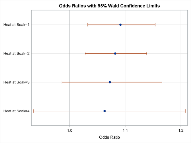
The ODDSRATIO statement produces the "Odds Ratio Estimates and Wald Confidence Intervals" table (Figure 53.6), and a graphical display of these estimates is shown in Figure 53.7. The differences between the odds ratios are small compared to the variability shown by their confidence intervals, which confirms the previous conclusion that the Heat*Soak parameter is not significantly different from zero.
| Odds Ratio Estimates and Wald Confidence Intervals | |||
|---|---|---|---|
| Label | Estimate | 95% Confidence Limits | |
| Heat at Soak=1 | 1.091 | 1.032 | 1.154 |
| Heat at Soak=2 | 1.082 | 1.028 | 1.139 |
| Heat at Soak=3 | 1.072 | 0.986 | 1.166 |
| Heat at Soak=4 | 1.063 | 0.935 | 1.208 |
Since the Heat*Soak interaction is nonsignificant, the following statements fit a main-effects model:
proc logistic data=ingots;
   model r/n = Heat Soak;
run;
The results of this analysis are shown in the following figures. The model information and response profiles are the same as those in Figure 53.1 and Figure 53.2 for the saturated model. The "Model Fit Statistics" table in Figure 53.8 shows that the AIC and SC for the main-effects model are smaller than for the saturated model, indicating that the main-effects model might be the preferred model. As in the preceding model, the "Testing Global Null Hypothesis: BETA=0" table indicates that the parameters are significantly different from zero.
| Model Fit Statistics | |||
|---|---|---|---|
| Criterion | Intercept Only |
Intercept and Covariates |
With Constant |
| AIC | 108.988 | 101.346 | 34.080 |
| SC | 112.947 | 113.221 | 45.956 |
| -2 Log L | 106.988 | 95.346 | 28.080 |
| Testing Global Null Hypothesis: BETA=0 | |||
|---|---|---|---|
| Test | Chi-Square | DF | Pr > ChiSq |
| Likelihood Ratio | 11.6428 | 2 | 0.0030 |
| Score | 15.1091 | 2 | 0.0005 |
| Wald | 13.0315 | 2 | 0.0015 |
The "Analysis of Maximum Likelihood Estimates" table in Figure 53.9 again shows that the Soak parameter is not significantly different from zero (p=0.8639). The odds ratio for each effect parameter, estimated by exponentiating the corresponding parameter estimate, is shown in the "Odds Ratios Estimates" table (Figure 53.9), along with 95% Wald confidence intervals. The confidence interval for the Soak parameter contains the value 1, which also indicates that this effect is not significant.
| Analysis of Maximum Likelihood Estimates | |||||
|---|---|---|---|---|---|
| Parameter | DF | Estimate | Standard Error |
Wald Chi-Square |
Pr > ChiSq |
| Intercept | 1 | -5.5592 | 1.1197 | 24.6503 | <.0001 |
| Heat | 1 | 0.0820 | 0.0237 | 11.9454 | 0.0005 |
| Soak | 1 | 0.0568 | 0.3312 | 0.0294 | 0.8639 |
| Odds Ratio Estimates | |||
|---|---|---|---|
| Effect | Point Estimate | 95% Wald Confidence Limits |
|
| Heat | 1.085 | 1.036 | 1.137 |
| Soak | 1.058 | 0.553 | 2.026 |
| Association of Predicted Probabilities and Observed Responses |
|||
|---|---|---|---|
| Percent Concordant | 64.4 | Somers' D | 0.460 |
| Percent Discordant | 18.4 | Gamma | 0.555 |
| Percent Tied | 17.2 | Tau-a | 0.028 |
| Pairs | 4500 | c | 0.730 |
Using these parameter estimates, you can calculate the estimated logit of  as
as
 |
For example, if Heat 7 and Soak1, then logit
 . Using this logit estimate, you can calculate
  as follows:
 |
This gives the predicted probability of the event (ingot not ready for rolling) for Heat7 and Soak1. Note that PROC LOGISTIC can calculate these statistics for you; use the OUTPUT statement with the PREDICTED= option, or use the SCORE statement.
To illustrate the use of an alternative form of input data, the following program creates the ingots data set with the new variables NotReady and Freq instead of n and r. The variable NotReady represents the response of individual units; it has a value of 1 for units not ready for rolling (event) and a value of 0 for units ready for rolling (nonevent). The variable Freq represents the frequency of occurrence of each combination of Heat, Soak, and NotReady. Note that, compared to the previous data set, NotReady1 implies Freqr, and NotReady0 implies Freqn–r.
data ingots;
   input Heat Soak NotReady Freq @@;
   datalines;
7 1.0 0 10  14 1.0 0 31  14 4.0 0 19  27 2.2 0 21  51 1.0 1  3
7 1.7 0 17  14 1.7 0 43  27 1.0 1  1  27 2.8 1  1  51 1.0 0 10
7 2.2 0  7  14 2.2 1  2  27 1.0 0 55  27 2.8 0 21  51 1.7 0  1
7 2.8 0 12  14 2.2 0 31  27 1.7 1  4  27 4.0 1  1  51 2.2 0  1
7 4.0 0  9  14 2.8 0 31  27 1.7 0 40  27 4.0 0 15  51 4.0 0  1
;
The following statements invoke PROC LOGISTIC to fit the main-effects model by using the alternative form of the input data set:
proc logistic data=ingots;
   model NotReady(event='1') = Heat Soak;
   freq Freq;
run;
Results of this analysis are the same as the preceding single-trial main-effects analysis. The displayed output for the two runs are identical except for the background information of the model fit and the "Response Profile" table shown in Figure 53.10.
| Response Profile | ||
|---|---|---|
| Ordered Value |
NotReady | Total Frequency |
| 1 | 0 | 375 |
| 2 | 1 | 12 |
By default, Ordered Values are assigned to the sorted response values in ascending order, and PROC LOGISTIC models the probability of the response level that corresponds to the Ordered Value 1. There are several methods to change these defaults; the preceding statements specify the response variable option EVENT= to model the probability of NotReady=1 as displayed in Figure 53.10. See the section Response Level Ordering for more details.