The LOGISTIC Procedure
- Overview
- Getting Started
-
Syntax
 PROC LOGISTIC Statement BY Statement CLASS Statement CONTRAST Statement EFFECT Statement EFFECTPLOT Statement ESTIMATE Statement EXACT Statement EXACTOPTIONS Statement FREQ Statement LSMEANS Statement LSMESTIMATE Statement MODEL Statement ODDSRATIO Statement OUTPUT Statement ROC Statement ROCCONTRAST Statement SCORE Statement SLICE Statement STORE Statement STRATA Statement TEST Statement UNITS Statement WEIGHT Statement
 -
Details
Missing Values Response Level Ordering Link Functions and the Corresponding Distributions Determining Observations for Likelihood Contributions Iterative Algorithms for Model Fitting Convergence Criteria Existence of Maximum Likelihood Estimates Effect-Selection Methods Model Fitting Information Generalized Coefficient of Determination Score Statistics and Tests Confidence Intervals for Parameters Odds Ratio Estimation Rank Correlation of Observed Responses and Predicted Probabilities Linear Predictor, Predicted Probability, and Confidence Limits Classification Table Overdispersion The Hosmer-Lemeshow Goodness-of-Fit Test Receiver Operating Characteristic Curves Testing Linear Hypotheses about the Regression Coefficients Regression Diagnostics Scoring Data Sets Conditional Logistic Regression Exact Conditional Logistic Regression Input and Output Data Sets Computational Resources Displayed Output ODS Table Names ODS Graphics
-
Examples
Stepwise Logistic Regression and Predicted Values Logistic Modeling with Categorical Predictors Ordinal Logistic Regression Nominal Response Data: Generalized Logits Model Stratified Sampling Logistic Regression Diagnostics ROC Curve, Customized Odds Ratios, Goodness-of-Fit Statistics, R-Square, and Confidence Limits Comparing Receiver Operating Characteristic Curves Goodness-of-Fit Tests and Subpopulations Overdispersion Conditional Logistic Regression for Matched Pairs Data Firth’s Penalized Likelihood Compared with Other Approaches Complementary Log-Log Model for Infection Rates Complementary Log-Log Model for Interval-Censored Survival Times Scoring Data Sets Using the LSMEANS Statement
- References
| Conditional Logistic Regression |
The method of maximum likelihood described in the preceding sections relies on large-sample asymptotic normality for the validity of estimates and especially of their standard errors. When you do not have a large sample size compared to the number of parameters, this approach might be inappropriate and might result in biased inferences. This situation typically arises when your data are stratified and you fit intercepts to each stratum so that the number of parameters is of the same order as the sample size. For example, in a  matched pairs study with
  pairs and
  covariates, you would estimate
  intercept parameters and slope parameters. Taking the stratification into account by "conditioning out" (and not estimating) the stratum-specific intercepts gives consistent and asymptotically normal MLEs for the slope coefficients. See Breslow and Day (1980) and Stokes, Davis, and Koch (2000) for more information. If your nuisance parameters are not just stratum-specific intercepts, you can perform an exact conditional logistic regression .
Computational Details
For each stratum  ,
,  , number the observations as
  so that
  indexes the
  th observation in the th stratum. Denote the covariates for observation as
  and its binary response as
  , and let
  ,
,  , and
, and  . Let the dummy variables
  , be indicator functions for the strata (
 if the observation is in stratum ), and denote
  for observation ,
  , and
, and  . Denote
  ) and
) and  . Arrange the observations in each stratum so that
  for
for  , and
, and  for
for  . Suppose all observations have unit frequency.
Consider the binary logistic regression model written as
 |
where the parameter vector  consists of
  ,
,  is the intercept for stratum
  , and
, and  is the parameter vector for the covariates.
From the section Determining Observations for Likelihood Contributions, you can write the likelihood contribution of observation  as
as
 |
where when the response takes Ordered Value 1, and otherwise.
The full likelihood is
 |
Unconditional likelihood inference is based on maximizing this likelihood function.
When your nuisance parameters are the stratum-specific intercepts  , and the slopes are your parameters of interest, "conditioning out" the nuisance parameters produces the conditional likelihood (Lachin; 2000)
 |
where the summation is over all  subsets
  of
of  observations chosen from the
  observations in stratum . Note that the nuisance parameters have been factored out of this equation.
For conditional asymptotic inference, maximum likelihood estimates  of the regression parameters are obtained by maximizing the conditional likelihood, and asymptotic results are applied to the conditional likelihood function and the maximum likelihood estimators. A relatively fast method of computing this conditional likelihood and its derivatives is given by Gail, Lubin, and Rubinstein (1981) and Howard (1972). The default optimization techniques, which are the same as those implemented by the NLP procedure in SAS/OR software, are as follows:
Newton-Raphson with ridging when the number of parameters

quasi-Newton when

conjugate gradient when

Sometimes the log likelihood converges but the estimates diverge. This condition is flagged by having inordinately large standard errors for some of your parameter estimates, and can be monitored by specifying the ITPRINT option. Unfortunately, broad existence criteria such as those discussed in the section Existence of Maximum Likelihood Estimates do not exist for this model. It might be possible to circumvent such a problem by standardizing your independent variables before fitting the model.
Regression Diagnostic Details
Diagnostics are used to indicate observations that might have undue influence on the model fit or that might be outliers. Further investigation should be performed before removing such an observation from the data set.
The derivations in this section use an augmentation method described by Storer and Crowley (1985), which provides an estimate of the "one-step" DFBETAS estimates advocated by Pregibon (1984). The method also provides estimates of conditional stratum-specific predicted values, residuals, and leverage for each observation. The augmentation method can take a lot of time and memory.
Following Storer and Crowley (1985), the log-likelihood contribution can be written as
 |
 |
 |
|||
 |
|
 |
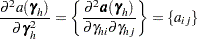
and the subscript on matrices indicates the submatrix for the stratum,  , and
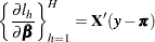
, and  . Then the gradient and information matrix are
 |
|
 |
|||
 |
|
 |
where
 |
|
 |
|||
 |
|
 |
|||
 |
|
 |
|||
 |
|
 |
and where  is the conditional stratum-specific probability that subject in stratum is a case, the summation on
  is over all subsets from
  of size that contain the index , and the summation on
  is over all subsets from of size that contain the indices and
  .
.
To produce the true one-step estimate  , start at the MLE , delete the th observation, and use this reduced data set to compute the next Newton-Raphson step. Note that if there is only one event or one nonevent in a stratum, deletion of that single observation is equivalent to deletion of the entire stratum. The augmentation method does not take this into account.
The augmented model is
 |
where  has a
has a  in the th coordinate, and use
  as the initial estimate for
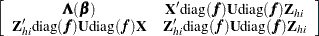
  . The gradient and information matrix before the step are
 |
|
 |
|||
 |
|
 |
Inserting the  and
and  into the Gail, Lubin, and Rubinstein (1981) algorithm provides the appropriate estimates of
  and
and  . Indicate these estimates with
  ,
,  ,
,  , and
, and  .
.
DFBETA is computed from the information matrix as
 |
|
 |
|||
 |
|
 |
|||
|
|
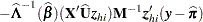 |
where
 |
|
 |
For each observation in the data set, a DFBETA statistic is computed for each parameter  ,
,  , and standardized by the standard error of from the full data set to produce the estimate of DFBETAS.
The estimated leverage is defined as
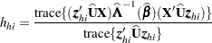 |
This definition of leverage produces different values from those defined by Pregibon (1984), Moolgavkar, Lustbader, and Venzon (1985), and Hosmer and Lemeshow (2000); however, it has the advantage that no extra computations beyond those for the DFBETAS are required.
The estimated residuals  are obtained from
  , and the weights, or predicted probabilities, are then
  . The residuals are standardized and reported as (estimated) Pearson residuals:
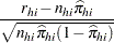 |
where  is the number of events in the observation and
  is the number of trials.
The STDRES option in the INFLUENCE and PLOTS=INFLUENCE options computes the standardized Pearson residual:
 |
For events/trials MODEL statement syntax, treat each observation as two observations (the first for the nonevents and the second for the events) with frequencies  and
and  , and augment the model with a matrix
 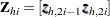 instead of a single
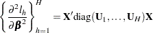
  vector. Writing
  in the preceding section results in the following gradient and information matrix:
|
|
 |
|||
|
|
 |
The predicted probabilities are then  , while the leverage and the DFBETAS are produced from in a fashion similar to that for the preceding single-trial equations.