The LOGISTIC Procedure
- Overview
- Getting Started
-
Syntax
 PROC LOGISTIC Statement BY Statement CLASS Statement CONTRAST Statement EFFECT Statement EFFECTPLOT Statement ESTIMATE Statement EXACT Statement EXACTOPTIONS Statement FREQ Statement LSMEANS Statement LSMESTIMATE Statement MODEL Statement ODDSRATIO Statement OUTPUT Statement ROC Statement ROCCONTRAST Statement SCORE Statement SLICE Statement STORE Statement STRATA Statement TEST Statement UNITS Statement WEIGHT Statement
 -
Details
Missing Values Response Level Ordering Link Functions and the Corresponding Distributions Determining Observations for Likelihood Contributions Iterative Algorithms for Model Fitting Convergence Criteria Existence of Maximum Likelihood Estimates Effect-Selection Methods Model Fitting Information Generalized Coefficient of Determination Score Statistics and Tests Confidence Intervals for Parameters Odds Ratio Estimation Rank Correlation of Observed Responses and Predicted Probabilities Linear Predictor, Predicted Probability, and Confidence Limits Classification Table Overdispersion The Hosmer-Lemeshow Goodness-of-Fit Test Receiver Operating Characteristic Curves Testing Linear Hypotheses about the Regression Coefficients Regression Diagnostics Scoring Data Sets Conditional Logistic Regression Exact Conditional Logistic Regression Input and Output Data Sets Computational Resources Displayed Output ODS Table Names ODS Graphics
-
Examples
Stepwise Logistic Regression and Predicted Values Logistic Modeling with Categorical Predictors Ordinal Logistic Regression Nominal Response Data: Generalized Logits Model Stratified Sampling Logistic Regression Diagnostics ROC Curve, Customized Odds Ratios, Goodness-of-Fit Statistics, R-Square, and Confidence Limits Comparing Receiver Operating Characteristic Curves Goodness-of-Fit Tests and Subpopulations Overdispersion Conditional Logistic Regression for Matched Pairs Data Firth’s Penalized Likelihood Compared with Other Approaches Complementary Log-Log Model for Infection Rates Complementary Log-Log Model for Interval-Censored Survival Times Scoring Data Sets Using the LSMEANS Statement
- References
| Receiver Operating Characteristic Curves |
ROC curves are used to evaluate and compare the performance of diagnostic tests; they can also be used to evaluate model fit. An ROC curve is just a plot of the proportion of true positives (events predicted to be events) versus the proportion of false positives (nonevents predicted to be events).
In a sample of  individuals, suppose
  individuals are observed to have a certain condition or event. Let this group be denoted by
  , and let the group of the remaining
  individuals who do not have the condition be denoted by
  . Risk factors are identified for the sample, and a logistic regression model is fitted to the data. For the
  th individual, an estimated probability
  of the event of interest is calculated. Note that the are computed as shown in the section Linear Predictor, Predicted Probability, and Confidence Limits and are not the cross validated estimates discussed in the section Classification Table.
Suppose the individuals undergo a test for predicting the event and the test is based on the estimated probability of the event. Higher values of this estimated probability are assumed to be associated with the event. A receiver operating characteristic (ROC) curve can be constructed by varying the cutpoint that determines which estimated event probabilities are considered to predict the event. For each cutpoint  , the following measures can be output to a data set by specifying the OUTROC= option in the MODEL statement or the OUTROC= option in the SCORE statement:
 |
 |
 |
|||
 |
|
 |
|||
 |
|
 |
|||
 |
|
 |
|||
 |
 |
 |
|||
 |
|
 |
where  is the indicator function.
Note that _POS_() is the number of correctly predicted event responses, _NEG_() is the number of correctly predicted nonevent responses, _FALPOS_() is the number of falsely predicted event responses, _FALNEG_() is the number of falsely predicted nonevent responses, _SENSIT_() is the sensitivity of the test, and _1MSPEC_() is one minus the specificity of the test.
The ROC curve is a plot of sensitivity (_SENSIT_) against 1–specificity (_1MSPEC_). The plot can be produced by using the PLOTS option or by using the GPLOT or SGPLOT procedure with the OUTROC= data set. See Example 53.7 for an illustration. The area under the ROC curve, as determined by the trapezoidal rule, is estimated by the concordance index, c, in the "Association of Predicted Probabilities and Observed Responses" table.
Comparing ROC Curves
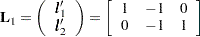
ROC curves can be created from each model fit in a selection routine, from the specified model in the MODEL statement, from specified models in ROC statements, or from input variables which act as  in the preceding discussion. Association statistics are computed for these models, and the models are compared when the ROCCONTRAST statement is specified. The ROC comparisons are performed by using a contrast matrix to take differences of the areas under the empirical ROC curves (DeLong, DeLong, and Clarke-Pearson; 1988). For example, if you have three curves and the second curve is the reference, the contrast used for the overall test is
 |
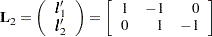
and you can optionally estimate and test each row of this contrast, in order to test the difference between the reference curve and each of the other curves. If you do not want to use a reference curve, the global test optionally uses the following contrast:
 |
You can also specify your own contrast matrix. Instead of estimating the rows of these contrasts, you can request that the difference between every pair of ROC curves be estimated and tested.
By default for the reference contrast, the specified or selected model is used as the reference unless the NOFIT option is specified in the MODEL statement, in which case the first ROC model is the reference.
In order to label the contrasts, a name is attached to every model. The name for the specified or selected model is the MODEL statement label, or "Model" if the MODEL label is not present. The ROC statement models are named with their labels, or as "ROC " for the th ROC statement if a label is not specified. The contrast
  is labeled as "Reference = ModelName", where ModelName is the reference model name, while
  is labeled "Adjacent Pairwise Differences". The estimated rows of the contrast matrix are labeled "ModelName1 – ModelName2". In particular, for the rows of , ModelName2 is the reference model name. If you specify your own contrast matrix, then the contrast is labeled "Specified" and the th contrast row estimates are labeled "Row".
If ODS Graphics is enabled, then all ROC curves are displayed individually and are also overlaid in a final display. If a selection method is specified, then the curves produced in each step of the model selection process are overlaid onto a single plot and are labeled "Step", and the selected model is displayed on a separate plot and on a plot with curves from specified ROC statements. See Example 53.8 for an example.
ROC Computations
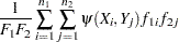
The trapezoidal area under an empirical ROC curve is equal to the Mann-Whitney two-sample rank measure of association statistic (a generalized  -statistic) applied to two samples,
  , in and
  , in . PROC LOGISTIC uses the predicted probabilities in place of
  and
and  ; however, in general any criterion could be used. Denote the frequency of observation in
  as
as  , and denote the total frequency in as
  . The WEIGHTED option replaces with
  , where
  is the weight of observation in group . The trapezoidal area under the curve is computed as
 |
|
 |
|||
 |
|
 |
so that  . Note that the concordance index,
  , in the "Association of Predicted Probabilities and Observed Responses" table is computed by creating 500 bins and binning the
  and
and  ; this results in more ties than the preceding method (unless the BINWIDTH=0 or ROCEPS=0 option is specified), so is not necessarily equal to
  .
.
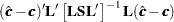
To compare  empirical ROC curves, first compute the trapezoidal areas. Asymptotic normality of the estimated area follows from -statistic theory, and a covariance matrix
  can be computed; see DeLong, DeLong, and Clarke-Pearson (1988) for details. A Wald confidence interval for the
  th area,
  , can be constructed as
 |
where  is the th diagonal of .
For a contrast of ROC curve areas,  , the statistic
 |
has a chi-square distribution with df rank(
rank( ). For a row of the contrast,
  ,
,
 |
has a standard normal distribution. The corresponding confidence interval is
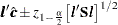 |