The TRANSREG Procedure
- Overview
-
Getting Started

-
Syntax
-
DetailsModel Statement UsageBox-Cox TransformationsUsing Splines and KnotsScoring Spline VariablesLinear and Nonlinear Regression FunctionsSimultaneously Fitting Two Regression FunctionsPenalized B-SplinesSmoothing SplinesSmoothing Splines Changes and EnhancementsIteration History Changes and EnhancementsANOVA CodingsMissing ValuesMissing Values, UNTIE, and Hypothesis TestsControlling the Number of IterationsUsing the REITERATE Algorithm OptionAvoiding Constant TransformationsConstant VariablesCharacter OPSCORE VariablesConvergence and DegeneraciesImplicit and Explicit InterceptsPassive ObservationsPoint ModelsRedundancy AnalysisOptimal ScalingOPSCORE, MONOTONE, UNTIE, and LINEAR TransformationsSPLINE and MSPLINE TransformationsSpecifying the Number of KnotsSPLINE, BSPLINE, and PSPLINE ComparisonsHypothesis TestsOutput Data SetOUTTEST= Output Data SetComputational ResourcesUnbalanced ANOVA without CLASS VariablesHypothesis Tests for Simple Univariate ModelsHypothesis Tests with Monotonicity ConstraintsHypothesis Tests with Dependent Variable TransformationsHypothesis Tests with One-Way ANOVAUsing the DESIGN Output OptionDiscrete Choice Experiments: DESIGN, NORESTORE, NOZEROCenteringDisplayed OutputODS Table NamesODS Graphics
-
Examples
- References
PROC TRANSREG can fit curves through data and detect nonlinear relationships among variables. This example uses a subset of
the data from an experiment in which nitrogen oxide emissions from a single cylinder engine are measured for various combinations
of fuel and equivalence ratio (Brinkman, 1981). This gas data set is available from the Sashelp library. The following step creates a subset of the data for analysis:
title 'Gasoline and Emissions Data';

data gas;
   set sashelp.gas;
   if fuel in ('Ethanol', '82rongas', 'Gasohol');
run;
The next step fits a spline or curve through the data and displays the regression results. For information about splines and knots, see the sections Smoothing Splines, Linear and Nonlinear Regression Functions, Simultaneously Fitting Two Regression Functions, and Using Splines and Knots, as well as Example 101.1. The following statements produce Figure 101.1:
ods graphics on;

* Request a Spline Transformation of Equivalence Ratio;
proc transreg data=Gas solve ss2 plots=(transformation obp residuals);
   model identity(nox) = spline(EqRatio / nknots=4);
   where fuel in ('Ethanol', '82rongas', 'Gasohol');
run;
The SOLVE algorithm option, or a-option, requests a direct solution for both the transformation and the parameter estimates. For many models, PROC TRANSREG with
the SOLVE a-option can produce exact results without iteration. The SS2 (Type II sums of squares) a-option requests regression and ANOVA results. The PLOTS= option requests plots of the variable transformations, a plot of the observed values by the predicted values, and a plot
of the residuals. The dependent variable NOx was specified with an IDENTITY transformation, which means that it will not be transformed, just as in ordinary regression. The independent variable EqRatio, in contrast, is transformed by using a cubic spline with four knots. The NKNOTS= option is known as a transformation option, or t-option. Graphical results are enabled when ODS Graphics is enabled. The results are shown in Figure 101.1 through Figure 101.5.
Figure 101.1: Iteration, ANOVA, and Regression Results
| Gasoline and Emissions Data |
| Dependent Variable Identity(NOx) Nitrogen Oxide |
| Number of Observations Read | 112 |
|---|---|
| Number of Observations Used | 110 |
| TRANSREG MORALS Algorithm Iteration History for Identity(NOx) | |||||
|---|---|---|---|---|---|
| Iteration Number |
Average Change |
Maximum Change |
R-Square | Criterion Change |
Note |
| 0 | 1.04965 | 3.46121 | 0.00917 | ||
| 1 | 0.00000 | 0.00000 | 0.82429 | 0.81512 | Converged |
| Algorithm converged. |
| The TRANSREG Procedure Hypothesis Tests for Identity(NOx) Nitrogen Oxide |
| Univariate ANOVA Table Based on the Usual Degrees of Freedom | |||||
|---|---|---|---|---|---|
| Source | DF | Sum of Squares | Mean Square | F Value | Pr > F |
| Model | 7 | 180.0951 | 25.72788 | 68.36 | <.0001 |
| Error | 102 | 38.3891 | 0.37636 | ||
| Corrected Total | 109 | 218.4842 | |||
| Root MSE | 0.61348 | R-Square | 0.8243 |
|---|---|---|---|
| Dependent Mean | 2.25022 | Adj R-Sq | 0.8122 |
| Coeff Var | 27.26334 |
| Univariate Regression Table Based on the Usual Degrees of Freedom | |||||||
|---|---|---|---|---|---|---|---|
| Variable | DF | Coefficient | Type II Sum of Squares |
Mean Square | F Value | Pr > F | Label |
| Intercept | 1 | 8.3165407 | 324.065 | 324.065 | 861.04 | <.0001 | Intercept |
| Spline(EqRatio) | 7 | -6.5740158 | 180.095 | 25.728 | 68.36 | <.0001 | Equivalence Ratio |
PROC TRANSREG increases the squared multiple correlation from the original value of 0.00917 to 0.82429. Iteration 0 shows
the fit before the data are transformed, and iteration 1 shows the fit after the transformation, which was directly solved
for in the initial iteration. The change values for iteration 0 show the change from the original EqRatio variable to the transformed EqRatio variable. For this model, no improvement on the initial solution is possible, so in iteration 1, all change values are zero.
The ANOVA and regression results show that you are fitting a model with 7 model parameters, 4 knots plus a degree 3 or cubic
spline. The overall model fit is identical to the test for the spline transformation, since there is only one term in the
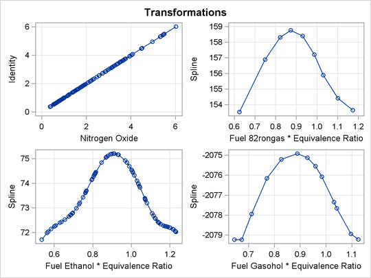
model besides the intercept, and the results are significant at the 0.0001 level. The transformations are shown next in Figure 101.2.
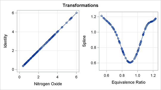
The transformation plots show the identity transformation of NOx and the nonlinear spline transformation of EqRatio. These plots are requested with the PLOTS=TRANSFORMATION option. The plot on the left shows that NOx is unchanged, which is always the case with the IDENTITY transformation. In contrast, the spline transformation of EqRatio is nonlinear. It is this nonlinear transformation of EqRatio that accounts for the increase in fit that is shown in the iteration history table.
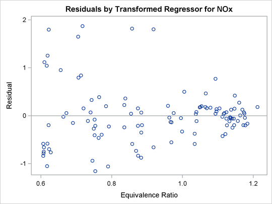
The residuals plot in Figure 101.3 shows the residuals as a function of the transformed independent variable.
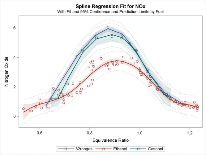
The “Spline Regression Fit” plot in Figure 101.4 displays the nonlinear regression function plotted through the original data, along with 95% confidence and prediction limits. This plot clearly shows that nitrous oxide emissions are largest in the middle range of equivalence ratio, 0.08 to 1.0, and are much lower for the extreme values of equivalence ratio, such as around 0.6 and 1.2.
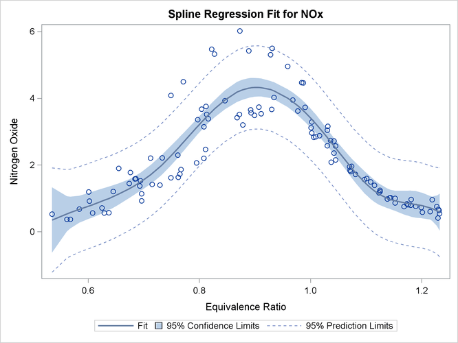
This plot is produced by default when ODS Graphics is enabled and when there is an IDENTITY dependent variable and one non-CLASS
independent variable. The plot consists of an ordinary scatter plot of NOx plotted as a function of EqRatio. It also contains the predicted values of NOx, which are a function of the spline transformation of EqRatio (or TEqRatio shown previously), and are plotted as a function of EqRatio. Similarly, it contains confidence limits based on NOx and TEqRatio.
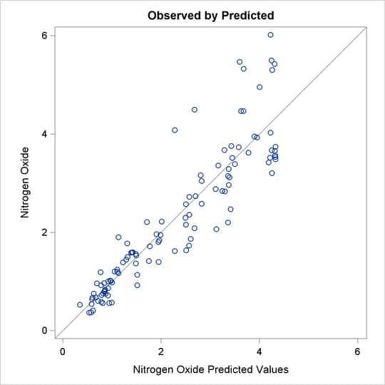
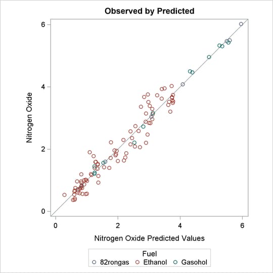
The “Observed by Predicted” values plot in Figure 101.5 displays the dependent variable plotted as a function of the regression predicted values along with a linear regression line,
which for this plot always has a slope of 1. This plot was requested with the OBP or OBSERVEDBYPREDICTED suboption in the
PLOTS= option. The residual differences between the transformed data and the regression line show how well the nonlinearly transformed
data fit a linear-regression model. The residuals look mostly random; however, they are larger for larger values of NOx, suggesting that maybe this is not the optimal model. You can also see this by examining the fit of the function through
the original scatter plot in Figure 101.4. Near the middle of the function, the residuals are much larger. You can refit the model, this time requesting separate functions
for each type of fuel. You can request the original scatter plot, without any regression information and before the variables
are transformed, by specifying the SCATTER suboption in the PLOTS= option.
These next statements fit an additive model with separate functions for each of the different fuels. The statements produce Figure 101.6 through Figure 101.9.
* Separate Curves and Intercepts;
proc transreg data=Gas solve ss2 additive plots=(transformation obp);
   model identity(nox) = class(Fuel / zero=none) |
                         spline(EqRatio / nknots=4 after);
run;
The ADDITIVE a-option requests an additive model, where the regression coefficients are absorbed into the transformations, and so the final regression
coefficients are all one. The specification CLASS(Fuel / ZERO=NONE) recodes fuel into a set of three binary variables, one for each of the three fuels in this data set. The vertical bar between
the CLASS and SPLINE specifications request both main effects and interactions. For this model, it requests both a separate intercept and a separate
spline function for each fuel. The original two variables, Fuel and EqRatio, are replaced by six variables—three binary intercept terms and three spline variables. The three spline variables are zero
when their corresponding intercept binary variable is zero, and nonzero otherwise. The nonzero parts are optimally transformed
by the analysis. The AFTER t-option specified with the SPLINE transformation specifies that the four knots should be selected independently for each of the three
spline transformations, after EqRatio is crossed with the CLASS variable. Alternatively, and by default, the knots are chosen by examining EqRatio before it is crossed with the CLASS variable, and the same knots are used for all three transformations. The results are
shown in Figure 101.6.
Figure 101.6: Iteration, ANOVA, and Regression Results
| Gasoline and Emissions Data |
| Dependent Variable Identity(NOx) Nitrogen Oxide |
| Class Level Information | ||
|---|---|---|
| Class | Levels | Values |
| Fuel | 3 | 82rongas Ethanol Gasohol |
| Number of Observations Read | 112 |
|---|---|
| Number of Observations Used | 110 |
| Implicit Intercept Model |
| TRANSREG MORALS Algorithm Iteration History for Identity(NOx) | |||||
|---|---|---|---|---|---|
| Iteration Number |
Average Change |
Maximum Change |
R-Square | Criterion Change |
Note |
| 0 | 0.12476 | 1.13866 | 0.18543 | ||
| 1 | 0.00000 | 0.00000 | 0.95870 | 0.77327 | Converged |
| Algorithm converged. |
| Hypothesis Test Iterations Excluding Spline(Fuel82rongasEqRatio) | |||||
|---|---|---|---|---|---|
| TRANSREG MORALS Algorithm Iteration History for Identity(NOx) | |||||
| Iteration Number |
Average Change |
Maximum Change |
R-Square | Criterion Change |
Note |
| 0 | 0.00000 | 0.00000 | 0.80234 | ||
| 1 | 0.00000 | 0.00000 | 0.80234 | -.00000 | Converged |
| Algorithm converged. |
| Hypothesis Test Iterations Excluding Spline(FuelEthanolEqRatio) | |||||
|---|---|---|---|---|---|
| TRANSREG MORALS Algorithm Iteration History for Identity(NOx) | |||||
| Iteration Number |
Average Change |
Maximum Change |
R-Square | Criterion Change |
Note |
| 0 | 0.00000 | 0.00000 | 0.48801 | ||
| 1 | 0.00000 | 0.00000 | 0.48801 | -.00000 | Converged |
| Algorithm converged. |
| Hypothesis Test Iterations Excluding Spline(FuelGasoholEqRatio) | |||||
|---|---|---|---|---|---|
| TRANSREG MORALS Algorithm Iteration History for Identity(NOx) | |||||
| Iteration Number |
Average Change |
Maximum Change |
R-Square | Criterion Change |
Note |
| 0 | 0.00000 | 0.00000 | 0.80052 | ||
| 1 | 0.00000 | 0.00000 | 0.80052 | -.00000 | Converged |
| Algorithm converged. |
| The TRANSREG Procedure Hypothesis Tests for Identity(NOx) Nitrogen Oxide |
| Univariate ANOVA Table Based on the Usual Degrees of Freedom | |||||
|---|---|---|---|---|---|
| Source | DF | Sum of Squares | Mean Square | F Value | Pr > F |
| Model | 23 | 209.4613 | 9.107012 | 86.80 | <.0001 |
| Error | 86 | 9.0229 | 0.104918 | ||
| Corrected Total | 109 | 218.4842 | |||
| Root MSE | 0.32391 | R-Square | 0.9587 |
|---|---|---|---|
| Dependent Mean | 2.25022 | Adj R-Sq | 0.9477 |
| Coeff Var | 14.39461 |
| Univariate Regression Table Based on the Usual Degrees of Freedom | |||||||
|---|---|---|---|---|---|---|---|
| Variable | DF | Coefficient | Type II Sum of Squares |
Mean Square | F Value | Pr > F | Label |
| Class.Fuel82rongas | 1 | 1.00000000 | 32.634 | 32.6338 | 311.04 | <.0001 | Fuel 82rongas |
| Class.FuelEthanol | 1 | 1.00000000 | 97.406 | 97.4058 | 928.40 | <.0001 | Fuel Ethanol |
| Class.FuelGasohol | 1 | 1.00000000 | 34.672 | 34.6720 | 330.47 | <.0001 | Fuel Gasohol |
| Spline(Fuel82rongasEqRatio) | 7 | 1.00000000 | 34.162 | 4.8803 | 46.52 | <.0001 | Fuel 82rongas * Equivalence Ratio |
| Spline(FuelEthanolEqRatio) | 7 | 1.00000000 | 102.840 | 14.6914 | 140.03 | <.0001 | Fuel Ethanol * Equivalence Ratio |
| Spline(FuelGasoholEqRatio) | 7 | 1.00000000 | 34.561 | 4.9372 | 47.06 | <.0001 | Fuel Gasohol * Equivalence Ratio |
| ZERO=SUM and ZERO=NONE coefficient tests are not exact when there are iterative transformations. Those tests are performed holding all transformations fixed, and so are generally liberal. |
The first iteration history table in Figure 101.6 shows that PROC TRANSREG increases the squared multiple correlation from the original value of 0.18543 to 0.95870. The remaining iteration histories pertain to PROC TRANSREG’s process of comparing models to test hypotheses. The important thing to look for is convergence in all of the tables.
The transformations, shown in Figure 101.7, show that for all three groups, the transformation of EqRatio is approximately quadratic.
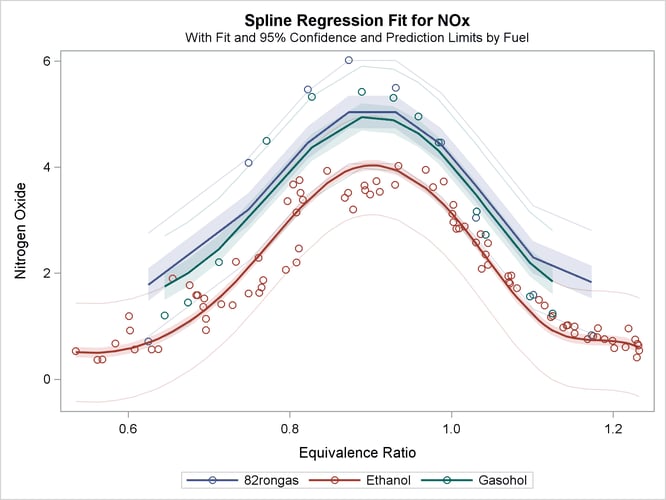
The fit plot, shown in Figure 101.8, shows that there are in fact three distinct functions in the data. The increase in fit over the previous model comes from individually fitting each group instead of providing an aggregate fit.
The residuals in the observed by predicted plot displayed in Figure 101.9 are much better for this analysis.
You could fit a model that is “in between” the two models shown previously. This next model provides for separate intercepts for each group, but calls for a common function. There are still three functions, one per group, but their shapes are the same, and they are equidistant or parallel. This model is requested by omitting the vertical bar so that separate intercepts are requested, but not separate curves within each group. The following statements fit the separate intercepts model and create Figure 101.10:
* Separate Intercepts;
proc transreg data=Gas solve ss2 additive;
   model identity(nox) = class(Fuel / zero=none)
                         spline(EqRatio / nknots=4);
run;
The ANOVA table and fit plot are shown in Figure 101.10.
Figure 101.10: Separate Intercepts Only
| Gasoline and Emissions Data |
| Univariate ANOVA Table Based on the Usual Degrees of Freedom | |||||
|---|---|---|---|---|---|
| Source | DF | Sum of Squares | Mean Square | F Value | Pr > F |
| Model | 9 | 196.7548 | 21.86165 | 100.61 | <.0001 |
| Error | 100 | 21.7294 | 0.21729 | ||
| Corrected Total | 109 | 218.4842 | |||
Now, squared multiple correlation is 0.9005, which is smaller than the model with the unconstrained separate curves, but larger than the model with only one curve. Because of the restrictions on the shapes, these curves do not track the data as well as the previous model. However, this model is more parsimonious with many fewer parameters.
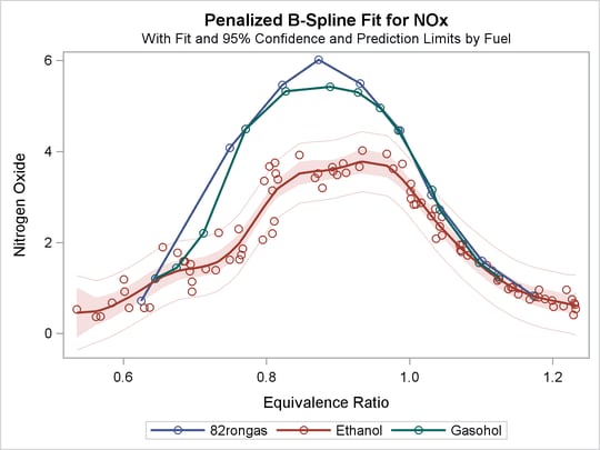
There are other ways to fit curves through scatter plots in PROC TRANSREG. For example, you could use smoothing splines or penalized B-splines, as is illustrated next. The following statements fit separate curves through each group by using penalized B-splines and produce Figure 101.11:
* Separate Curves and Intercepts with Penalized B-Splines;
proc transreg data=Gas ss2 plots=transformation lprefix=0;
   model identity(nox) = class(Fuel / zero=none) * pbspline(EqRatio);
run;
This example asks for a separate penalized B-spline transformation, PBSPLINE, of equivalence ratio for each type of fuel. The LPREFIX=0 a-option is specified in the PROC statement so that zero characters of the CLASS variable name (Fuel) are used in constructing the labels for the coded variables. The result is label components like “Ethanol” instead of the more redundant “Fuel Ethanol”. The results of this analysis are shown in Figure 101.11.
| Dependent Variable Identity(NOx) Nitrogen Oxide |
| Class Level Information | ||
|---|---|---|
| Class | Levels | Values |
| Fuel | 3 | 82rongas Ethanol Gasohol |
| Number of Observations Read | 112 |
|---|---|
| Number of Observations Used | 110 |
| Implicit Intercept Model |
| TRANSREG Univariate Algorithm Iteration History for Identity(NOx) |
|||
|---|---|---|---|
| Iteration Number |
Average Change |
Maximum Change |
Note |
| 1 | 0.00000 | 0.00000 | Converged |
| Algorithm converged. |
| The TRANSREG Procedure Hypothesis Tests for Identity(NOx) Nitrogen Oxide |
| Univariate ANOVA Table, Penalized B-Spline Transformation | |||||
|---|---|---|---|---|---|
| Source | DF | Sum of Squares | Mean Square | F Value | Pr > F |
| Model | 33.194 | 211.4818 | 6.371106 | 68.97 | <.0001 |
| Error | 75.806 | 7.0024 | 0.092373 | ||
| Corrected Total | 109 | 218.4842 | |||
| Root MSE | 0.30393 | R-Square | 0.9680 |
|---|---|---|---|
| Dependent Mean | 2.25022 | Adj R-Sq | 0.9539 |
| Coeff Var | 13.50663 |
| Penalized B-Spline Transformation | |||||
|---|---|---|---|---|---|
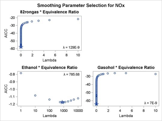
| Variable | DF | Coefficient | Lambda | AICC | Label |
| Pbspline(Fuel82rongasEqRatio) | 9.000 | 1.000 | 1.287E-7 | -57.7841 | 82rongas * Equivalence Ratio |
| Pbspline(FuelEthanolEqRatio) | 12.19 | 1.000 | 785.7 | -1.1736 | Ethanol * Equivalence Ratio |
| Pbspline(FuelGasoholEqRatio) | 13.00 | 1.000 | 7.019E-9 | -64.2961 | Gasohol * Equivalence Ratio |
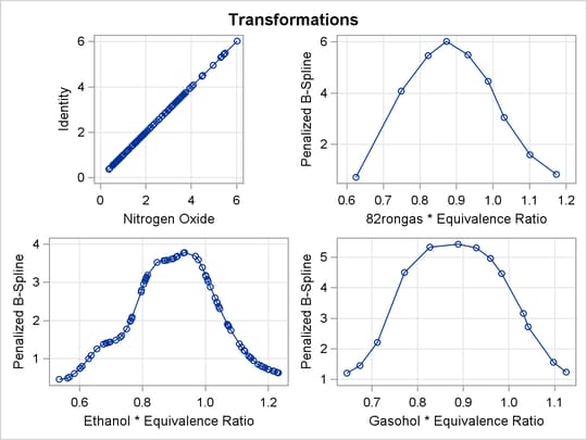
With penalized B-splines, the degrees of freedom are based on the trace of the transformation hat matrix and are typically not integers. The first panel of plots shows AICC as a function of lambda, the smoothing parameter. The smoothing parameter is automatically chosen, and since the smoothing parameters range from essentially 0 to almost 800, it is clear that some functions are smoother than others. The plots of the criterion (AICC in this example) as a function of lambda use a linear scale for the horizontal axis when the range of lambdas is small, as in the first and third plot, and a log scale when the range is large, as in the second plot. The transformation for equivalence ratio for Ethanol required more smoothing than for the other two fuels. All three have an overall quadratic shape, but for Ethanol, the function more closely follows the smaller variations in the data. You could get similar results with SPLINE by using more knots.
For other examples of curve fitting by using PROC TRANSREG, see the sections Smoothing Splines, Linear and Nonlinear Regression Functions, Simultaneously Fitting Two Regression Functions, and Using Splines and Knots, as well as Example 101.3. These examples include cases where multiple curves are fit through scatter plots with multiple groups. Special cases include linear models with separate slopes and separate intercepts. Many constraints on the slopes, curves, and intercepts are possible.