The TRANSREG Procedure
- Overview
-
Getting Started

-
Syntax
-
DetailsModel Statement UsageBox-Cox TransformationsUsing Splines and KnotsScoring Spline VariablesLinear and Nonlinear Regression FunctionsSimultaneously Fitting Two Regression FunctionsPenalized B-SplinesSmoothing SplinesSmoothing Splines Changes and EnhancementsIteration History Changes and EnhancementsANOVA CodingsMissing ValuesMissing Values, UNTIE, and Hypothesis TestsControlling the Number of IterationsUsing the REITERATE Algorithm OptionAvoiding Constant TransformationsConstant VariablesCharacter OPSCORE VariablesConvergence and DegeneraciesImplicit and Explicit InterceptsPassive ObservationsPoint ModelsRedundancy AnalysisOptimal ScalingOPSCORE, MONOTONE, UNTIE, and LINEAR TransformationsSPLINE and MSPLINE TransformationsSpecifying the Number of KnotsSPLINE, BSPLINE, and PSPLINE ComparisonsHypothesis TestsOutput Data SetOUTTEST= Output Data SetComputational ResourcesUnbalanced ANOVA without CLASS VariablesHypothesis Tests for Simple Univariate ModelsHypothesis Tests with Monotonicity ConstraintsHypothesis Tests with Dependent Variable TransformationsHypothesis Tests with One-Way ANOVAUsing the DESIGN Output OptionDiscrete Choice Experiments: DESIGN, NORESTORE, NOZEROCenteringDisplayed OutputODS Table NamesODS Graphics
-
Examples
- References
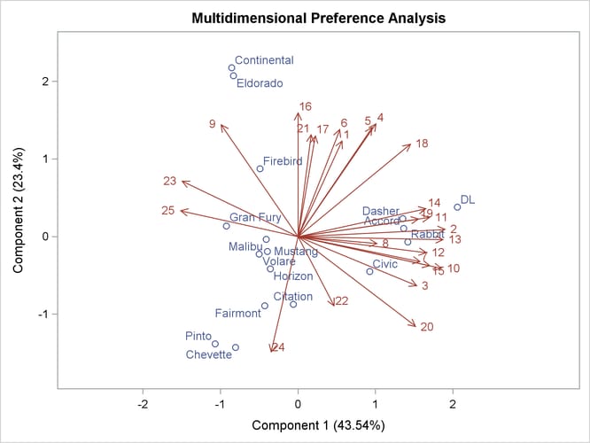
This example uses PROC TRANSREG to perform a preference mapping (PREFMAP) analysis (Carroll, 1972) of automobile preference data after a PROC PRINQUAL principal component analysis. The PREFMAP analysis is a response surface regression that locates ideal points for each dependent variable in a space defined by the independent variables.
The data are ratings obtained from 25 judges of their preference for each of 17 automobiles. The ratings were made on a scale
of zero (very weak preference) to nine (very strong preference). These judgments were made in 1980 about that year’s products.
There are two character variables that indicate the manufacturer and model of the automobile. The data set also contains three
ratings: miles per gallon (MPG), projected reliability (Reliability), and quality of the ride (Ride). These ratings are on a scale of one (bad) to five (good). PROC PRINQUAL creates an OUT= data set containing standardized principal component scores (Prin1 and Prin2), along with the ID variables Model, MPG, Reliability, and Ride.
While this data set contains all of the information needed for the subsequent preference mapping, you can make slightly more
informative plots by adding new variable labels to the principal component score variables. The default labels are ’Component
1’, ’Component 2’, and so on. These are by necessity rather generic since they are created before any data are read, and they
must be appropriate across BY groups when a BY variable is specified. In contrast, the MDPREF plot in PROC PRINQUAL has axis
labels of the form ’Component 1 (43.54%)’ and ’Component 2 (23.4%)’ that show the proportion of variance accounted for by
each component. You can create an output data set from the MDPREF plot by using the ODS OUTPUT statement and then use only
the label information from it to reset the labels in the output data set from PROC PRINQUAL. In the DATA PLOT step, the SET
statement for the MD data set is specified before the SET statement for the PRESULTS data set. The if 0 ensures that no data are actually read from it, but nevertheless the properties of the Prin1 and Prin2 variables including the variable labels are set based on the properties of those variables in the MD data set.
The first PROC TRANSREG step fits univariate regression models for MPG and Reliability. All variables are designated IDENTITY. A vector drawn in the plot of Prin1 and Prin2 from the origin to the point defined by an attribute’s regression coefficients approximately shows how the autos differ on
that attribute. See Carroll (1972) for more information. The Prin1 and Prin2 columns of the TResult1 OUT= data set contain the automobile coordinates (_Type_=’SCORE’ observations) and endpoints of the MPG and Reliability vectors (_Type_=’M COEFFI’ observations).
The second PROC TRANSREG step fits a univariate regression model with Ride designated IDENTITY, and Prin1 and Prin2 designated POINT. The POINT expansion creates an additional independent variable _ISSQ_, which contains the sum of Prin1 squared and Prin2 squared. The OUT= data set TResult2 contains no _Type_=’SCORE’ observations, only ideal point (_Type_=’M POINT’) coordinates for Ride. The coordinates of both the vectors and the ideal points are output by specifying COORDINATES in the OUTPUT statement in PROC TRANSREG.
A vector model is used for MPG and Reliability because perfectly efficient and reliable automobiles do not exist in the data set. The ideal points for MPG and Reliability are far removed from the plot of the automobiles. It is more likely that an ideal point for quality of the ride is in the
plot, so an ideal point model is used for the ride variable. See Carroll (1972) and Schiffman, Reynolds, and Young (1981) for discussions of the vector model and point models (including the EPOINT and QPOINT versions of the point model that are not used in this example). For the vector model, the default coordinates stretch factor
of 2.5 was used. This extends the vectors by a factor of 2.5 from their standard lengths, making a better graphical display.
Sometimes the default vectors are short and near the origin, and they look better when they are extended.
The following statements produce Output 101.6.1 through Output 101.6.5:
title 'Preference Ratings for Automobiles Manufactured in 1980';

options validvarname=any;

data CarPreferences;
   input Make $ 1-10 Model $ 12-22 @25 ('1'n-'25'n) (1.)
         MPG Reliability Ride;
   datalines;
Cadillac   Eldorado     8007990491240508971093809 3 2 4
Chevrolet  Chevette     0051200423451043003515698 5 3 2
Chevrolet  Citation     4053305814161643544747795 4 1 5
Chevrolet  Malibu       6027400723121345545668658 3 3 4
Ford       Fairmont     2024006715021443530648655 3 3 4
Ford       Mustang      5007197705021101850657555 3 2 2
Ford       Pinto        0021000303030201500514078 4 1 1
Honda      Accord       5956897609699952998975078 5 5 3
Honda      Civic        4836709507488852567765075 5 5 3
Lincoln    Continental  7008990592230409962091909 2 4 5
Plymouth   Gran Fury    7006000434101107333458708 2 1 5
Plymouth   Horizon      3005005635461302444675655 4 3 3
Plymouth   Volare       4005003614021602754476555 2 1 3
Pontiac    Firebird     0107895613201206958265907 1 1 5
Volkswagen Dasher       4858696508877795377895000 5 3 4
Volkswagen Rabbit       4858509709695795487885000 5 4 3
Volvo      DL           9989998909999987989919000 4 5 5
;
ods graphics on;

* Compute Coordinates for a 2-Dimensional Scatter Plot of Automobiles;
proc prinqual data=CarPreferences out=PResults(drop='1'n-'25'n)
              n=2 replace standard scores mdpref=2;
   id Model MPG Reliability Ride;
   transform identity('1'n-'25'n);
   title2 'Multidimensional Preference (MDPREF) Analysis';
   ods output mdprefplot=md;
run;

options validvarname=v7;

title2 'Preference Mapping (PREFMAP) Analysis';

* Add the Labels from the Plot to the Results Data Set;
data plot;
   if 0 then set md(keep=prin:);
   set presults;
run;

* Compute Endpoints for MPG and Reliability Vectors;
proc transreg data=plot rsquare;
   Model identity(MPG Reliability)=identity(Prin1 Prin2);
   output tstandard=center coordinates replace out=TResult1;
   id Model;
run;

* Compute Ride Ideal Point Coordinates;
proc transreg data=plot rsquare;
   Model identity(Ride)=point(Prin1 Prin2);
   output tstandard=center coordinates replace noscores out=TResult2;
   id Model;
run;

proc print;
run;
Output 101.6.1: Preference Ratings Example Output
| Preference Ratings for Automobiles Manufactured in 1980 |
| Multidimensional Preference (MDPREF) Analysis |
| PRINQUAL MTV Algorithm Iteration History | |||||
|---|---|---|---|---|---|
| Iteration Number |
Average Change |
Maximum Change |
Proportion of Variance |
Criterion Change |
Note |
| 1 | 0.00000 | 0.00000 | 0.66946 | Converged | |
| Algorithm converged. |
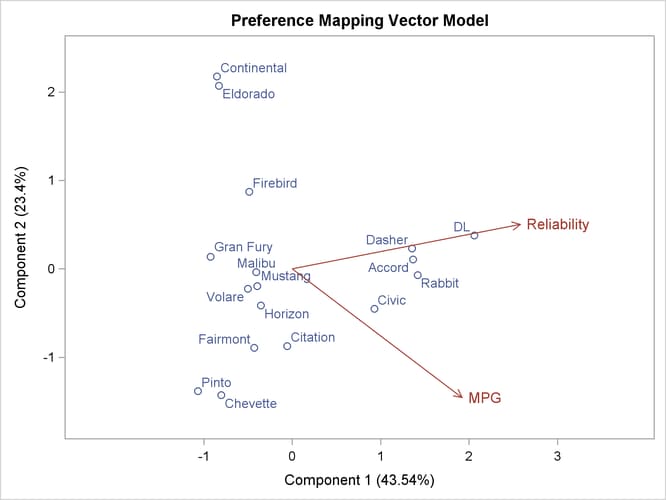
Output 101.6.3 shows that an unreliable-to-reliable direction extends from the left and slightly below the origin to the right and slightly
above the origin. The Japanese and European automobiles are rated, on the average, as more reliable. A low MPG to good MPG direction extends from the top left of the plot to the bottom right. The smaller automobiles, on the average, get better
gas mileage.
Output 101.6.3: Preference Mapping Vector Plot
| Preference Ratings for Automobiles Manufactured in 1980 |
| Preference Mapping (PREFMAP) Analysis |
| The TRANSREG Procedure Hypothesis Tests for Identity(MPG) |
| R-Square | 0.5720 |
|---|
| The TRANSREG Procedure Hypothesis Tests for Identity(Reliability) |
| R-Square | 0.5086 |
|---|
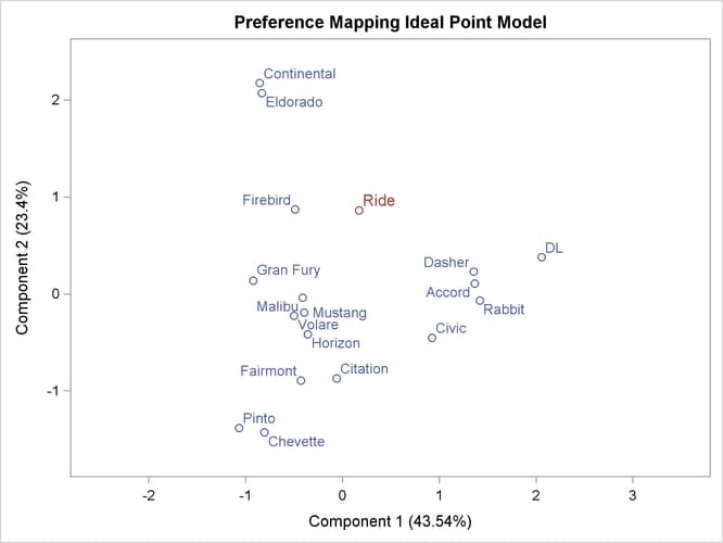
The ideal point for Ride in Output 101.6.4 is in the top, just right of the center of the plot. Automobiles near the Ride ideal point tend to have a better ride than automobiles far away. It can be seen from the R squares that none of these ratings
perfectly fits the model, so all of the interpretations are approximate.
Output 101.6.4: Preference Mapping Ideal Point Plot
| Preference Ratings for Automobiles Manufactured in 1980 |
| Preference Mapping (PREFMAP) Analysis |
| The TRANSREG Procedure Hypothesis Tests for Identity(Ride) |
| R-Square | 0.3780 |
|---|
The Ride point is a “negative-negative” ideal point. The point models assume that small ratings mean the object (automobile) is similar to the rating name and large
ratings imply dissimilarity to the rating name. Because the opposite scoring is used, the interpretation of the Ride point must be reversed to a negative ideal point (bad ride). However, the coefficient for the _ISSQ_ variable in Output 101.6.5 is negative, so the interpretation is reversed again, back to the original interpretation.
Output 101.6.5: Preference Mapping Ideal Point Coefficients
| Preference Ratings for Automobiles Manufactured in 1980 |
| Preference Mapping (PREFMAP) Analysis |
| Obs | _TYPE_ | _NAME_ | Ride | Intercept | Prin1 | Prin2 | _ISSQ_ | Model |
|---|---|---|---|---|---|---|---|---|
| 1 | M POINT | Ride | . | . | 0.49461 | 2.46539 | -0.17448 | Ride |