The TRANSREG Procedure
- Overview
-
Getting Started

-
Syntax
-
DetailsModel Statement UsageBox-Cox TransformationsUsing Splines and KnotsScoring Spline VariablesLinear and Nonlinear Regression FunctionsSimultaneously Fitting Two Regression FunctionsPenalized B-SplinesSmoothing SplinesSmoothing Splines Changes and EnhancementsIteration History Changes and EnhancementsANOVA CodingsMissing ValuesMissing Values, UNTIE, and Hypothesis TestsControlling the Number of IterationsUsing the REITERATE Algorithm OptionAvoiding Constant TransformationsConstant VariablesCharacter OPSCORE VariablesConvergence and DegeneraciesImplicit and Explicit InterceptsPassive ObservationsPoint ModelsRedundancy AnalysisOptimal ScalingOPSCORE, MONOTONE, UNTIE, and LINEAR TransformationsSPLINE and MSPLINE TransformationsSpecifying the Number of KnotsSPLINE, BSPLINE, and PSPLINE ComparisonsHypothesis TestsOutput Data SetOUTTEST= Output Data SetComputational ResourcesUnbalanced ANOVA without CLASS VariablesHypothesis Tests for Simple Univariate ModelsHypothesis Tests with Monotonicity ConstraintsHypothesis Tests with Dependent Variable TransformationsHypothesis Tests with One-Way ANOVAUsing the DESIGN Output OptionDiscrete Choice Experiments: DESIGN, NORESTORE, NOZEROCenteringDisplayed OutputODS Table NamesODS Graphics
-
Examples
- References
Box-Cox (1964) transformations are used to find potentially nonlinear transformations of a dependent variable. The Box-Cox transformation has the form
This family of transformations of the positive dependent variable y is controlled by the parameter ![]() . Transformations linearly related to square root, inverse, quadratic, cubic, and so on are all special cases. The limit as
. Transformations linearly related to square root, inverse, quadratic, cubic, and so on are all special cases. The limit as
![]() approaches 0 is the log transformation. More generally, Box-Cox transformations of the following form can be fit:
approaches 0 is the log transformation. More generally, Box-Cox transformations of the following form can be fit:
By default, c = 0. The parameter c can be used to rescale y so that it is strictly positive. By default, g = 1. Alternatively, g can be ![]() , where
, where ![]() is the geometric mean of y.
is the geometric mean of y.
The BOXCOX transformation in PROC TRANSREG can be used to perform a Box-Cox transformation of the dependent variable. You can specify
a list of power parameters by using the LAMBDA= t-option. By default, LAMBDA=–3 TO 3 BY 0.25. The procedure chooses the optimal power parameter by using a maximum likelihood criterion
(Draper and Smith 1981, pp. 225–226). You can specify the PARAMETER=c transformation option when you want to shift the values of y, usually to avoid negatives. To divide by ![]() , specify the GEOMETRICMEAN t-option.
, specify the GEOMETRICMEAN t-option.
Here are three examples of using the LAMBDA= t-option:
model BoxCox(y / lambda=0) = identity(x1-x5);
model BoxCox(y / lambda=-2 to 2 by 0.1) = identity(x1-x5);
model BoxCox(y) = identity(x1-x5);
Here is the first example:
model BoxCox(y / lambda=0) = identity(x1-x5);
LAMBDA=0 specifies a Box-Cox transformation with a power parameter of 0. Since a single value of 0 was specified for LAMBDA=, there is no difference between the following models:
model BoxCox(y / lambda=0) = identity(x1-x5);
model log(y) = identity(x1-x5);
Here is the second example:
model BoxCox(y / lambda=-2 to 2 by 0.1) = identity(x1-x5);
LAMBDA= specifies a list of power parameters. PROC TRANSREG tries each power parameter in the list and picks the best transformation. A maximum likelihood approach (Draper and Smith 1981, pp. 225–226) is used. With Box-Cox transformations, PROC TRANSREG finds the transformation before the usual iterations begin. Note that this is quite different from PROC TRANSREG’s usual approach of iteratively finding optimal transformations with ordinary and alternating least squares. It is analogous to SMOOTH and PBSPLINE, which also find transformations before the iterations begin based on a criterion other than least squares.
Here is the third example:
model BoxCox(y) = identity(x1-x5);
The default LAMBDA= list of –3 TO 3 BY 0.25 is used.
The procedure prints the optimal power parameter, a confidence interval on the power parameter (based on the ALPHA= t-option), a “convenient” power parameter (selected from the CLL= t-option list), and the log likelihood for each power parameter tried (see Example 101.2).
To illustrate how Box-Cox transformations work, data were generated from the model
where ![]() . The transformed data can be fit with a linear model
. The transformed data can be fit with a linear model
The following statements produce Figure 101.14 through Figure 101.15:
title 'Basic Box-Cox Example';

data x;
   do x = 1 to 8 by 0.025;
      y = exp(x + normal(7));
      output;
   end;
run;

ods graphics on;

title2 'Default Options';

proc transreg data=x test;
   model BoxCox(y) = identity(x);
run;
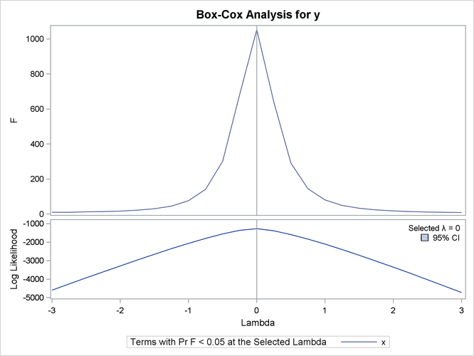
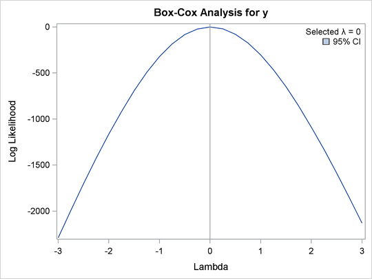
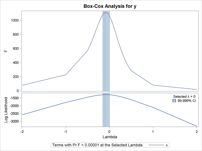
Figure 101.14 shows that PROC TRANSREG correctly selects the log transformation ![]() , with a narrow confidence interval. The
, with a narrow confidence interval. The ![]() plot shows that F is at its largest in the vicinity of the optimal Box-Cox transformation.
plot shows that F is at its largest in the vicinity of the optimal Box-Cox transformation.
The rest of the output, which contains the ANOVA results, is shown in Figure 101.15.
Figure 101.15: Basic Box-Cox Example, Default Output
| Dependent Variable BoxCox(y) |
| Number of Observations Read | 281 |
|---|---|
| Number of Observations Used | 281 |
| The TRANSREG Procedure Hypothesis Tests for BoxCox(y) |
| Univariate ANOVA Table Based on the Usual Degrees of Freedom | |||||
|---|---|---|---|---|---|
| Source | DF | Sum of Squares | Mean Square | F Value | Liberal p |
| Model | 1 | 1145.884 | 1145.884 | 1053.66 | >= <.0001 |
| Error | 279 | 303.421 | 1.088 | ||
| Corrected Total | 280 | 1449.305 | |||
| The above statistics are not adjusted for the fact that the dependent variable was transformed and so are generally liberal. | |||||
| Root MSE | 1.04285 | R-Square | 0.7906 |
|---|---|---|---|
| Dependent Mean | 4.49653 | Adj R-Sq | 0.7899 |
| Coeff Var | 23.19225 | Lambda | 0.0000 |
This next example uses several options. The LAMBDA= t-option specifies power parameters sparsely from –2 to –0.5 and 0.5 to 2 just to get the general shape of the log-likelihood function
in that region. Between –0.5 and 0.5, more power parameters are tried. The CONVENIENT t-option is specified so that if a power parameter like ![]() or
or ![]() is found in the confidence interval, it is used instead of the optimal power parameter. PARAMETER=2 is specified to add 2 to each y before performing the transformations. ALPHA=0.00001 specifies a wide confidence interval.
is found in the confidence interval, it is used instead of the optimal power parameter. PARAMETER=2 is specified to add 2 to each y before performing the transformations. ALPHA=0.00001 specifies a wide confidence interval.
These next statements perform the Box-Cox analysis and produce Figure 101.16 and Figure 101.17:
title2 'Several Options Demonstrated';

proc transreg data=x ss2 details
              plots=(transformation(dependent) scatter
                    observedbypredicted);
   model BoxCox(y / lambda=-2 -1 -0.5 to 0.5 by 0.05 1 2
                    convenient parameter=2 alpha=0.00001) =
         identity(x);
run;
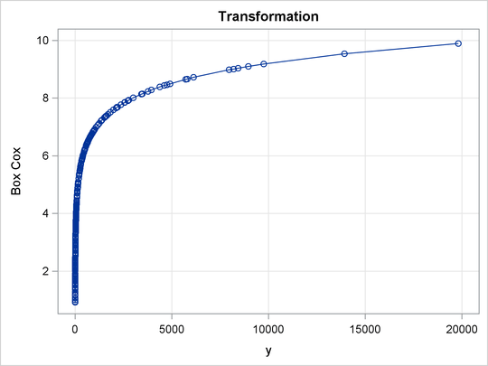
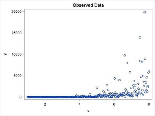
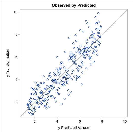
The results in Figure 101.16 and Figure 101.17 show that the optimal power parameter is –0.1, but 0 is in the confidence interval, and hence a log transformation is chosen. The actual Box-Cox transformation, the original scatter plot, and observed by predicted values plot are shown in Figure 101.17.
Figure 101.17: Basic Box-Cox Example, Several Options Demonstrated
| Dependent Variable BoxCox(y) |
| Number of Observations Read | 281 |
|---|---|
| Number of Observations Used | 281 |
| Model Statement Specification Details | ||||
|---|---|---|---|---|
| Type | DF | Variable | Description | Value |
| Dep | 1 | BoxCox(y) | Lambda Used | 0 |
| Lambda | -0.1 | |||
| Log Likelihood | -1280.1 | |||
| Conv. Lambda | 0 | |||
| Conv. Lambda LL | -1287.7 | |||
| CI Limit | -1289.9 | |||
| Alpha | 0.00001 | |||
| Parameter | 2 | |||
| Options | Convenient Lambda Used | |||
| Ind | 1 | Identity(x) | DF | 1 |
| The TRANSREG Procedure Hypothesis Tests for BoxCox(y) |
| Univariate ANOVA Table Based on the Usual Degrees of Freedom | |||||
|---|---|---|---|---|---|
| Source | DF | Sum of Squares | Mean Square | F Value | Liberal p |
| Model | 1 | 999.438 | 999.4381 | 1064.82 | >= <.0001 |
| Error | 279 | 261.868 | 0.9386 | ||
| Corrected Total | 280 | 1261.306 | |||
| The above statistics are not adjusted for the fact that the dependent variable was transformed and so are generally liberal. | |||||
| Root MSE | 0.96881 | R-Square | 0.7924 |
|---|---|---|---|
| Dependent Mean | 4.61429 | Adj R-Sq | 0.7916 |
| Coeff Var | 20.99591 | Lambda | 0.0000 |
| Univariate Regression Table Based on the Usual Degrees of Freedom | ||||||
|---|---|---|---|---|---|---|
| Variable | DF | Coefficient | Type II Sum of Squares |
Mean Square | F Value | Liberal p |
| Intercept | 1 | 0.42939328 | 8.746 | 8.746 | 9.32 | >= 0.0025 |
| Identity(x) | 1 | 0.92997620 | 999.438 | 999.438 | 1064.82 | >= <.0001 |
| The above statistics are not adjusted for the fact that the dependent variable was transformed and so are generally liberal. |
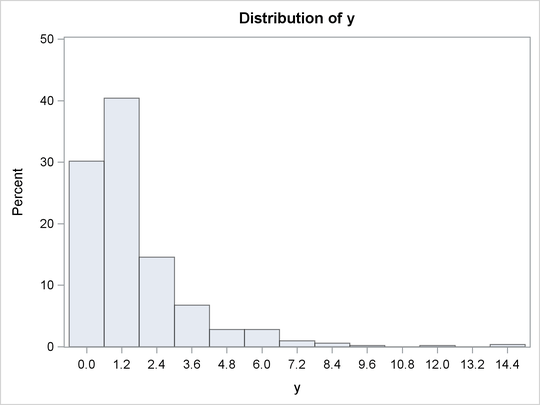
The next example shows how to find a Box-Cox transformation without an independent variable. This seeks to normalize the univariate
histogram. This example generates 500 random observations from a lognormal distribution. In addition, a constant variable
z is created that is all zero. This is because PROC TRANSREG requires some independent variable to be specified, even if it
is constant. Two options are specified in the PROC TRANSREG statement. MAXITER=0 is specified because the Box-Cox transformation is performed before any iterations are begun. No iterations are needed since
no other work is required. The NOZEROCONSTANT a-option (which can be abbreviated NOZ) is specified so that PROC TRANSREG does not print any warnings when it encounters the constant
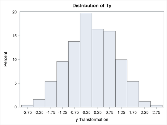
independent variable. The MODEL statement asks for a Box-Cox transformation of y and an IDENTITY transformation (which does nothing) of the constant variable z. Finally, PROC UNIVARIATE is run to show a histogram of the original variable y, and the Box-Cox transformation, Ty. The following statements fit the univariate Box-Cox model and produce Figure 101.18:
title 'Univariate Box-Cox';

data x;
   call streaminit(17);
   z = 0;
   do i = 1 to 500;
      y = rand('lognormal');
      output;
   end;
run;

proc transreg maxiter=0 nozeroconstant;
   model BoxCox(y) = identity(z);
   output;
run;

proc univariate noprint;
   histogram y ty;
run;
The PROC TRANSREG results in Figure 101.18 show that zero is chosen for lambda, so a log transformation is chosen. The first histogram shows that the original data are skewed, but a log transformation makes the data appear much more nearly normal.