The TRANSREG Procedure
- Overview
-
Getting Started

-
Syntax
-
DetailsModel Statement UsageBox-Cox TransformationsUsing Splines and KnotsScoring Spline VariablesLinear and Nonlinear Regression FunctionsSimultaneously Fitting Two Regression FunctionsPenalized B-SplinesSmoothing SplinesSmoothing Splines Changes and EnhancementsIteration History Changes and EnhancementsANOVA CodingsMissing ValuesMissing Values, UNTIE, and Hypothesis TestsControlling the Number of IterationsUsing the REITERATE Algorithm OptionAvoiding Constant TransformationsConstant VariablesCharacter OPSCORE VariablesConvergence and DegeneraciesImplicit and Explicit InterceptsPassive ObservationsPoint ModelsRedundancy AnalysisOptimal ScalingOPSCORE, MONOTONE, UNTIE, and LINEAR TransformationsSPLINE and MSPLINE TransformationsSpecifying the Number of KnotsSPLINE, BSPLINE, and PSPLINE ComparisonsHypothesis TestsOutput Data SetOUTTEST= Output Data SetComputational ResourcesUnbalanced ANOVA without CLASS VariablesHypothesis Tests for Simple Univariate ModelsHypothesis Tests with Monotonicity ConstraintsHypothesis Tests with Dependent Variable TransformationsHypothesis Tests with One-Way ANOVAUsing the DESIGN Output OptionDiscrete Choice Experiments: DESIGN, NORESTORE, NOZEROCenteringDisplayed OutputODS Table NamesODS Graphics
-
Examples
- References
Statistical procedures use ODS Graphics to create graphs as part of their output. ODS Graphics is described in detail in Chapter 21: Statistical Graphics Using ODS.
Before you create graphs, ODS Graphics must be enabled (for example, by specifying the ODS GRAPHICS ON statement). For more information about enabling and disabling ODS Graphics, see the section Enabling and Disabling ODS Graphics in Chapter 21: Statistical Graphics Using ODS.
The overall appearance of graphs is controlled by ODS styles. Styles and other aspects of using ODS Graphics are discussed in the section A Primer on ODS Statistical Graphics in Chapter 21: Statistical Graphics Using ODS.
Some graphs are produced by default; other graphs are produced by using statements and options. You can reference every graph produced through ODS Graphics with a name. The names of the graphs that PROC TRANSREG generates are listed in Table 101.8, along with the required statements and options.
Table 101.8: Graphs Produced by PROC TRANSREG
|
ODS Graph Name |
Plot Description |
Statement & Option |
|---|---|---|
|
BoxCoxFPlot |
Box-Cox |
MODEL & PROC, BOXCOX transform & PLOTS(UNPACK) |
|
BoxCoxLogLikePlot |
Box-Cox Log |
MODEL & PROC, BOXCOX transform & PLOTS(UNPACK) |
|
Box-Cox t or |
MODEL, BOXCOX transform |
|
|
BoxCoxtPlot |
Box-Cox t |
MODEL & PROC, BOXCOX transform & |
|
Simple Regression and Separate Group Regressions |
MODEL, a dependent variable that is not transformed, one non-CLASS independent variable, and at most one CLASS variable |
|
|
Dependent Variable by |
MODEL, PLOTS=OBSERVEDBYPREDICTED |
|
|
Penalized B-Spline |
MODEL, PBSPLINE transform |
|
|
Preference Mapping |
MODEL & PROC, IDENTITY transform & COORDINATES |
|
|
Preference Mapping |
MODEL & PROC, POINT expansion & COORDINATES |
|
|
Residuals |
PROC, PLOTS=RESIDUALS |
|
|
RMSEPlot |
Box-Cox Root Mean |
|
|
ScatterPlot |
Scatter Plot of Observed Data |
MODEL, one non-CLASS independent variable, and at most one CLASS variable, PLOTS=SCATTER |
|
Variable Transformations |
PROC, PLOTS=TRANSFORMATION |
This section illustrates one use of the PLOTS(INTERPOLATE) option for use with ODS Graphics. The data set has two groups of
observations, c = 1 and c = 2. Each group is sparse, having only five observations, so the plots of the transformations and fit functions are not smooth.
A second DATA step adds additional observations to the data set, over the range of x, with y missing. These observations do not contribute to the analysis, but they are used in computations of transformed and predicted
values. The resulting plots are much smoother in the latter case than in the former. The other results of the analysis are
the same. The following statements produce Figure 101.77 and Figure 101.78:
title 'Smoother Interpolation with PLOTS(INTERPOLATE)';

data a;
   input c y x;
   output;
   datalines;
1 1 1
1 2 2
1 4 3
1 6 4
1 7 5
2 3 1
2 4 2
2 5 3
2 4 4
2 5 5
;
ods graphics on;

proc transreg data=a plots=(tran fit) ss2;
   model ide(y) = pbs(x) * class(c / zero=none);
run;

data b;
   set a end=eof;
   output;
   if eof then do;
      y = .;
      do x = 1 to 5 by 0.05;
         c = 1; output;
         c = 2; output;
      end;
   end;
run;

proc transreg data=b plots(interpolate)=(tran fit) ss2;
   model ide(y) = pbs(x) * class(c / zero=none);
run;
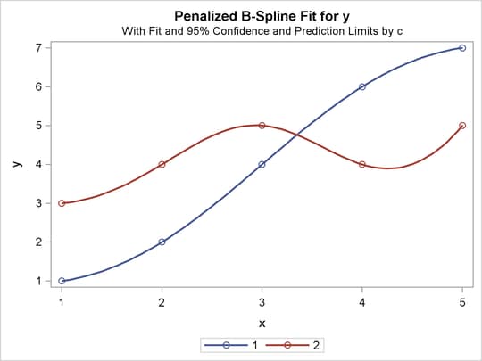
The results with no interpolation are shown in Figure 101.77. The transformation and fit functions are not at all smooth. The results with interpolation are shown in Figure 101.78. The transformation and fit functions are smooth in Figure 101.78, because there are intermediate points to plot.
Figure 101.77: No Interpolation
| Smoother Interpolation with PLOTS(INTERPOLATE) |
| Univariate ANOVA Table, Penalized B-Spline Transformation | |||||
|---|---|---|---|---|---|
| Source | DF | Sum of Squares | Mean Square | F Value | Pr > F |
| Model | 9 | 28.90000 | 3.211111 | Infty | <.0001 |
| Error | 12E-10 | 0.00000 | 0.000000 | ||
| Corrected Total | 9 | 28.90000 | |||
| Root MSE | 0 | R-Square | 1.0000 |
|---|---|---|---|
| Dependent Mean | 4.10000 | Adj R-Sq | 1.0000 |
| Coeff Var | 0 |
| Penalized B-Spline Transformation | |||||
|---|---|---|---|---|---|
| Variable | DF | Coefficient | Lambda | AICC | Label |
| Pbspline(xc1) | 5.0000 | 1.000 | 2.642E-7 | -66.4281 | x * c 1 |
| Pbspline(xc2) | 5.0000 | 1.000 | 2.516E-7 | -60.6430 | x * c 2 |
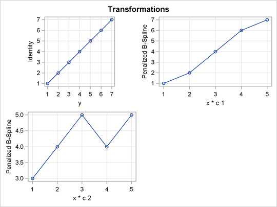
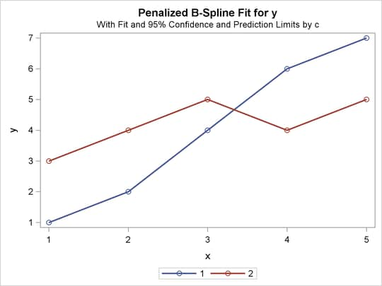
Figure 101.78: Interpolation with PLOTS(INTERPOLATE)
| Smoother Interpolation with PLOTS(INTERPOLATE) |
| Univariate ANOVA Table, Penalized B-Spline Transformation | |||||
|---|---|---|---|---|---|
| Source | DF | Sum of Squares | Mean Square | F Value | Pr > F |
| Model | 9 | 28.90000 | 3.211111 | Infty | <.0001 |
| Error | 12E-10 | 0.00000 | 0.000000 | ||
| Corrected Total | 9 | 28.90000 | |||
| Root MSE | 0 | R-Square | 1.0000 |
|---|---|---|---|
| Dependent Mean | 4.10000 | Adj R-Sq | 1.0000 |
| Coeff Var | 0 |
| Penalized B-Spline Transformation | |||||
|---|---|---|---|---|---|
| Variable | DF | Coefficient | Lambda | AICC | Label |
| Pbspline(xc1) | 5.0000 | 1.000 | 2.642E-7 | -66.4281 | x * c 1 |
| Pbspline(xc2) | 5.0000 | 1.000 | 2.516E-7 | -60.6430 | x * c 2 |