The TRANSREG Procedure
- Overview
-
Getting Started

-
Syntax
-
DetailsModel Statement UsageBox-Cox TransformationsUsing Splines and KnotsScoring Spline VariablesLinear and Nonlinear Regression FunctionsSimultaneously Fitting Two Regression FunctionsPenalized B-SplinesSmoothing SplinesSmoothing Splines Changes and EnhancementsIteration History Changes and EnhancementsANOVA CodingsMissing ValuesMissing Values, UNTIE, and Hypothesis TestsControlling the Number of IterationsUsing the REITERATE Algorithm OptionAvoiding Constant TransformationsConstant VariablesCharacter OPSCORE VariablesConvergence and DegeneraciesImplicit and Explicit InterceptsPassive ObservationsPoint ModelsRedundancy AnalysisOptimal ScalingOPSCORE, MONOTONE, UNTIE, and LINEAR TransformationsSPLINE and MSPLINE TransformationsSpecifying the Number of KnotsSPLINE, BSPLINE, and PSPLINE ComparisonsHypothesis TestsOutput Data SetOUTTEST= Output Data SetComputational ResourcesUnbalanced ANOVA without CLASS VariablesHypothesis Tests for Simple Univariate ModelsHypothesis Tests with Monotonicity ConstraintsHypothesis Tests with Dependent Variable TransformationsHypothesis Tests with One-Way ANOVAUsing the DESIGN Output OptionDiscrete Choice Experiments: DESIGN, NORESTORE, NOZEROCenteringDisplayed OutputODS Table NamesODS Graphics
-
Examples
- References
This section shows how to use PROC TRANSREG in simple regression (one dependent variable and one independent variable) to find the optimal regression line, a nonlinear but monotone regression function, and a nonlinear and nonmonotone regression function. To find a linear regression function, specify the IDENTITY transformation of the independent variable. For a monotone curve, specify the MSPLINE transformation of the independent variable. To relax the monotonicity constraint, specify the SPLINE transformation. You can get more flexibility in spline functions by specifying knots. The more knots you specify, the more freedom the function has to follow minor variations in the data. This example uses artificial data. While these artificial data are clearly not realistic, their distinct pattern helps illustrate how splines work. The following statements generate the data and produce Figure 101.28 through Figure 101.31:
title 'Linear and Nonlinear Regression Functions';

* Generate an Artificial Nonlinear Scatter Plot;
data a;
   do i = 1 to 500;
      x = i / 2.5;
      y = -((x/50)-1.5)**2 + sin(x/8) + sqrt(x)/5 + 2*log(x) + cos(x);
      x = x / 21;
      if y > 2 then output;
   end;
run;

ods graphics on;
ods select fitplot(persist);

title2 'Linear Regression';

proc transreg data=a;
   model identity(y)=identity(x);
run;

title2 'A Monotone Regression Function';

proc transreg data=a;
   model identity(y)=mspline(x / nknots=9);
run;

title2 'A Nonlinear Regression Function';

proc transreg data=a;
   model identity(y)=spline(x / nknots=9);
run;

title2 'A Nonlinear Regression Function, 100 Knots';

proc transreg data=a;
   model identity(y)=spline(x / nknots=100);
run;

ods select all;
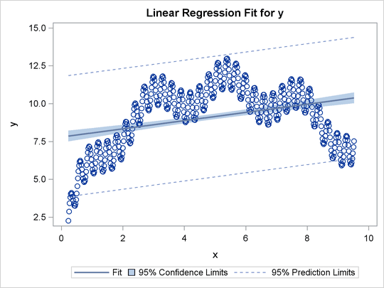
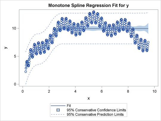
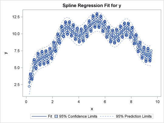
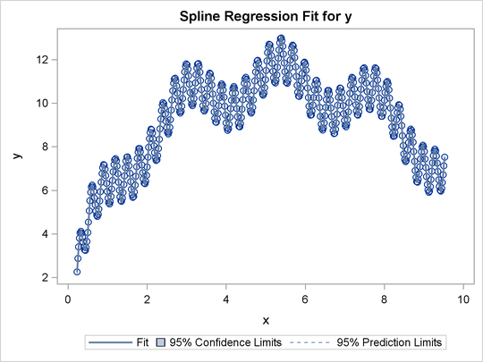
The squared correlation is only 0.15 for the linear regression in Figure 101.28. Clearly, a simple linear regression model is not appropriate for these data. By relaxing the constraints placed on the regression line, the proportion of variance accounted for increases from 0.15 (linear) to 0.61 (monotone in Figure 101.29) to 0.90 (nonlinear but smooth in Figure 101.30) to almost 1.0 with 100 knots (nonlinear and not very smooth in Figure 101.28). Relaxing the linearity constraint permits the regression function to bend and more closely follow the right portion of the scatter plot. Relaxing the monotonicity constraint permits the regression function to follow the periodic portion of the left side of the plot more closely. The nonlinear MSPLINE transformation is a quadratic spline with knots at the deciles. The first nonlinear nonmonotonic SPLINE transformation is a cubic spline with knots at the deciles.
Different knots and different degrees would produce slightly different results. The two nonlinear regression functions could be closely approximated by simpler piecewise linear regression functions. The monotone function could be approximated by a two-piece line with a single knot at the elbow. The first nonmonotone function could be approximated by a six-piece function with knots at the five elbows.
With this type of problem (one dependent variable with no missing values that is not transformed and one independent variable
that is nonlinearly transformed), PROC TRANSREG always iterates exactly twice (although only one iteration is necessary).
The first iteration reports the R square for the linear regression line and finds the optimal transformation of x. Since the data change in the first iteration, a second iteration is performed, which reports the R square for the final
nonlinear regression function, and zero data change. The predicted values, which are a linear function of the optimal transformation
of x, contain the Y coordinates for the nonlinear regression function. The variance of the predicted values divided by the variance
of y is the R square for the fit of the nonlinear regression function. When x is monotonically transformed, the transformation of x is always monotonically increasing, but the predicted values increase if the correlation is positive and decrease for negative
correlations.