The TRANSREG Procedure
- Overview
-
Getting Started

-
Syntax
-
DetailsModel Statement UsageBox-Cox TransformationsUsing Splines and KnotsScoring Spline VariablesLinear and Nonlinear Regression FunctionsSimultaneously Fitting Two Regression FunctionsPenalized B-SplinesSmoothing SplinesSmoothing Splines Changes and EnhancementsIteration History Changes and EnhancementsANOVA CodingsMissing ValuesMissing Values, UNTIE, and Hypothesis TestsControlling the Number of IterationsUsing the REITERATE Algorithm OptionAvoiding Constant TransformationsConstant VariablesCharacter OPSCORE VariablesConvergence and DegeneraciesImplicit and Explicit InterceptsPassive ObservationsPoint ModelsRedundancy AnalysisOptimal ScalingOPSCORE, MONOTONE, UNTIE, and LINEAR TransformationsSPLINE and MSPLINE TransformationsSpecifying the Number of KnotsSPLINE, BSPLINE, and PSPLINE ComparisonsHypothesis TestsOutput Data SetOUTTEST= Output Data SetComputational ResourcesUnbalanced ANOVA without CLASS VariablesHypothesis Tests for Simple Univariate ModelsHypothesis Tests with Monotonicity ConstraintsHypothesis Tests with Dependent Variable TransformationsHypothesis Tests with One-Way ANOVAUsing the DESIGN Output OptionDiscrete Choice Experiments: DESIGN, NORESTORE, NOZEROCenteringDisplayed OutputODS Table NamesODS Graphics
-
Examples
- References
The ENSO data set contains measurements of monthly averaged atmospheric pressure differences between Easter Island and Darwin,
Australia, for a period of 168 months (National Institute of Standards and Technology, 1998). The ENSO data set is available from the Sashelp library.
You can fit a curve through these data by using a penalized B-spline (Eilers and Marx, 1996) function and the following statements:
title 'Atmospheric Pressure Changes Between'
      ' Easter Island & Darwin, Australia';
ods graphics on;

proc transreg data=sashelp.enso;
   model identity(pressure) = pbspline(year);
run;
The dependent variable Pressure is specified along with an IDENTITY transformation, so Pressure is analyzed as is, with no transformations. The independent variable Year is specified with a PBSPLINE transformation, so a penalized B-spline model is fit. By default, a DEGREE=3 B-spline basis is used along with 100 evenly spaced knots and three evenly spaced exterior knots on each side of the data.
The penalized spline function is typically much smoother than you would get by using a SPLINE transformation or a BSPLINE expansion since changes in the coefficients of the basis are penalized to make a smoother fit. The output is shown next in
Output 101.3.1.
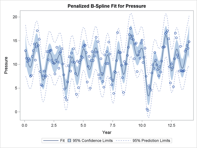
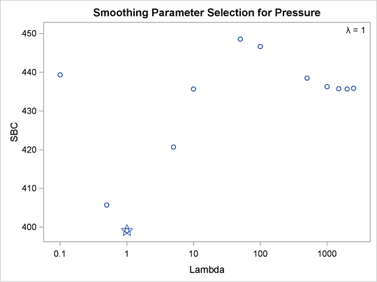
The results show a yearly cycle of pressure change. The procedure chose a smoothing parameter of ![]() . With data such as these, with many peaks and valleys, it might be useful to perform another analysis, this time asking for
a smoother plot. The Schwarz Bayesian criterion (SBC) is sometimes a better choice than the default criterion when you want a smoother plot. The following PROC TRANSREG step
requests a penalized B-spline analysis minimizing the SBC criterion:
. With data such as these, with many peaks and valleys, it might be useful to perform another analysis, this time asking for
a smoother plot. The Schwarz Bayesian criterion (SBC) is sometimes a better choice than the default criterion when you want a smoother plot. The following PROC TRANSREG step
requests a penalized B-spline analysis minimizing the SBC criterion:
proc transreg data=sashelp.enso;
   model identity(pressure) = pbspline(year / sbc);
run;
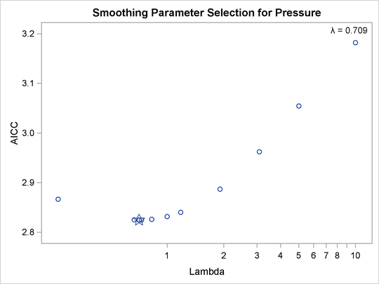
The plot of SBC as a function of ![]() is shown in Output 101.3.2.
is shown in Output 101.3.2.
The fit plot (not shown) is essentially the same as the one shown in Output 101.3.1 due to the similar choice of smoothing parameters: ![]() versus
versus ![]() . You can analyze these data again, this time forcing PROC TRANSREG to consider only larger smoothing parameters. The specification
LAMBDA=2 10000 RANGE eliminates from consideration the two lambdas that you previously saw and considers only
. You can analyze these data again, this time forcing PROC TRANSREG to consider only larger smoothing parameters. The specification
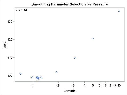
LAMBDA=2 10000 RANGE eliminates from consideration the two lambdas that you previously saw and considers only ![]() . The following statements produce Output 101.3.3:
. The following statements produce Output 101.3.3:
proc transreg data=sashelp.enso;
   model identity(pressure) = pbspline(year / sbc lambda=2 10000 range);
run;
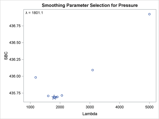
The results clearly show that there is a local minimum in the SBC(![]() ) function at
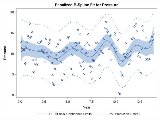
) function at ![]() . Using this lambda results in a much smoother regression function with a longer cycle than you saw previously. This second
cycle can be identified as the periodic warming of the Pacific Ocean known as “El Niño.” The SBC(
. Using this lambda results in a much smoother regression function with a longer cycle than you saw previously. This second
cycle can be identified as the periodic warming of the Pacific Ocean known as “El Niño.” The SBC(![]() ) function has at least two minima since there are at least two trends in the data. In the first analysis, PROC TRANSREG found
what is probably the globally optimal solution, and in the second set of analyses, with a little nudging away from the global
optimum, it found a very interesting locally optimal solution.
) function has at least two minima since there are at least two trends in the data. In the first analysis, PROC TRANSREG found
what is probably the globally optimal solution, and in the second set of analyses, with a little nudging away from the global
optimum, it found a very interesting locally optimal solution.
You can specify a list of lambdas to see SBC as a function of lambda over the range that includes both minima as follows:
proc transreg data=sashelp.enso;
   model identity(pressure) = pbspline(year / sbc lambda=.1 .5 1 5
                                       10 50 100 500 to 2500 by 500);
run;
The plot of SBC as a function of ![]() is shown in Output 101.3.4.
is shown in Output 101.3.4.