The TRANSREG Procedure
- Overview
-
Getting Started

-
Syntax
-
DetailsModel Statement UsageBox-Cox TransformationsUsing Splines and KnotsScoring Spline VariablesLinear and Nonlinear Regression FunctionsSimultaneously Fitting Two Regression FunctionsPenalized B-SplinesSmoothing SplinesSmoothing Splines Changes and EnhancementsIteration History Changes and EnhancementsANOVA CodingsMissing ValuesMissing Values, UNTIE, and Hypothesis TestsControlling the Number of IterationsUsing the REITERATE Algorithm OptionAvoiding Constant TransformationsConstant VariablesCharacter OPSCORE VariablesConvergence and DegeneraciesImplicit and Explicit InterceptsPassive ObservationsPoint ModelsRedundancy AnalysisOptimal ScalingOPSCORE, MONOTONE, UNTIE, and LINEAR TransformationsSPLINE and MSPLINE TransformationsSpecifying the Number of KnotsSPLINE, BSPLINE, and PSPLINE ComparisonsHypothesis TestsOutput Data SetOUTTEST= Output Data SetComputational ResourcesUnbalanced ANOVA without CLASS VariablesHypothesis Tests for Simple Univariate ModelsHypothesis Tests with Monotonicity ConstraintsHypothesis Tests with Dependent Variable TransformationsHypothesis Tests with One-Way ANOVAUsing the DESIGN Output OptionDiscrete Choice Experiments: DESIGN, NORESTORE, NOZEROCenteringDisplayed OutputODS Table NamesODS Graphics
-
Examples
- References
This example shows Box-Cox transformations with a yarn failure data set. For more information about Box-Cox transformations,
including using a Box-Cox transformation in a model with no independent variable, to normalize the distribution of the data,
see the section Box-Cox Transformations. In this example, a simple ![]() design was used to study the effects of different factors on the failure of a yarn manufacturing process. The design factors
are as follows:
design was used to study the effects of different factors on the failure of a yarn manufacturing process. The design factors
are as follows:
-
the length of test specimens of yarn, with levels of 250, 300, and 350 mm
-
the amplitude of the loading cycle, with levels of 8, 9, and 10 mmd
-
the load with levels of 40, 45, and 50 grams
The measured response was time (in cycles) until failure. However, you could just as well have measured the inverse of time until failure (in other words, the failure rate). Hence, the correct metric with which to analyze the response is not apparent. You can use PROC TRANSREG to find an optimum power transformation for the analysis. The following statements create the input SAS data set:
title 'Yarn Strength';

proc format;
   value a -1 =   8 0 =   9 1 =  10;
   value l -1 = 250 0 = 300 1 = 350;
   value o -1 =  40 0 =  45 1 =  50;
run;

data yarn;
   input Fail Amplitude Length Load @@;
   format amplitude a. length l. load o.;
   label fail = 'Time in Cycles until Failure';
   datalines;
 674 -1 -1 -1    370 -1 -1  0    292 -1 -1  1    338  0 -1 -1
 266  0 -1  0    210  0 -1  1    170  1 -1 -1    118  1 -1  0
  90  1 -1  1   1414 -1  0 -1   1198 -1  0  0    634 -1  0  1
1022  0  0 -1    620  0  0  0    438  0  0  1    442  1  0 -1
 332  1  0  0    220  1  0  1   3636 -1  1 -1   3184 -1  1  0
2000 -1  1  1   1568  0  1 -1   1070  0  1  0    566  0  1  1
1140  1  1 -1    884  1  1  0    360  1  1  1
;
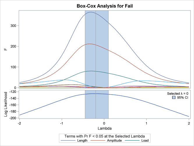
PROC TRANSREG is run to find the Box-Cox transformation. The lambda list is –2 TO 2 BY 0.05, which produces 81 lambdas, and
a convenient lambda is requested. This many power parameters makes a nice graphical display with plenty of detail around the
confidence interval. In the interest of space, only part of this table is displayed. The independent variables are designated
with the QPOINT expansion. QPOINT, for quadratic point model, gets its name from PROC TRANSREG’s ideal point modeling capabilities, which process variables
for a response surface analysis. What QPOINT does is create a set of independent variables consisting of the following: the m original variables (Length Amplitude Load), the m original variables squared (Length_2 Amplitude_2 Load_2), and the ![]() pairs of products between the m variables (
pairs of products between the m variables (LengthAmplitude LengthLoad AmplitudeLoad). The following statements produce Output 101.2.1:
ods graphics on;
proc transreg details data=yarn ss2
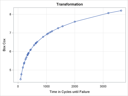
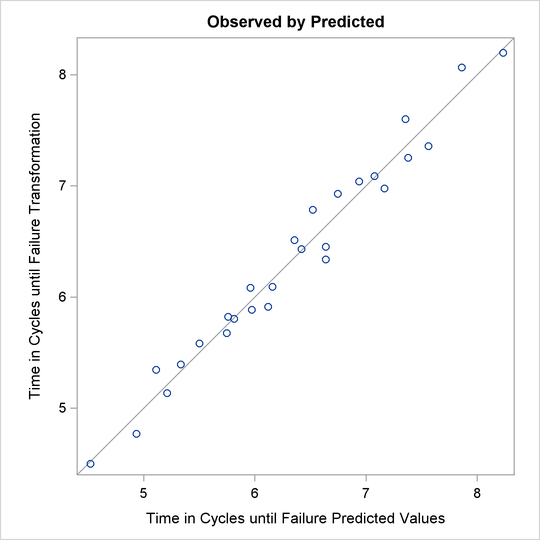
plots=(transformation(dependent) obp);
model BoxCox(fail / convenient lambda=-2 to 2 by 0.05) =
qpoint(length amplitude load);
run;
| Dependent Variable BoxCox(Fail) Time in Cycles until Failure |
| Number of Observations Read | 27 |
|---|---|
| Number of Observations Used | 27 |
| Model Statement Specification Details | ||||
|---|---|---|---|---|
| Type | DF | Variable | Description | Value |
| Dep | 1 | BoxCox(Fail) | Lambda Used | 0 |
| Lambda | -0.2 | |||
| Log Likelihood | -125.9 | |||
| Conv. Lambda | 0 | |||
| Conv. Lambda LL | -126.7 | |||
| CI Limit | -127.8 | |||
| Alpha | 0.05 | |||
| Options | Convenient Lambda Used | |||
| Label | Time in Cycles until Failure | |||
| Ind | 1 | Qpoint.Length | DF | 1 |
| Ind | 1 | Qpoint.Amplitude | DF | 1 |
| Ind | 1 | Qpoint.Load | DF | 1 |
| Ind | 1 | Qpoint.Length_2 | DF | 1 |
| Ind | 1 | Qpoint.Amplitude_2 | DF | 1 |
| Ind | 1 | Qpoint.Load_2 | DF | 1 |
| Ind | 1 | Qpoint.LengthAmplitude | DF | 1 |
| Ind | 1 | Qpoint.LengthLoad | DF | 1 |
| Ind | 1 | Qpoint.AmplitudeLoad | DF | 1 |
| The TRANSREG Procedure Hypothesis Tests for BoxCox(Fail) Time in Cycles until Failure |
| Univariate ANOVA Table Based on the Usual Degrees of Freedom | |||||
|---|---|---|---|---|---|
| Source | DF | Sum of Squares | Mean Square | F Value | Liberal p |
| Model | 9 | 22.56498 | 2.507220 | 66.73 | >= <.0001 |
| Error | 17 | 0.63871 | 0.037571 | ||
| Corrected Total | 26 | 23.20369 | |||
| The above statistics are not adjusted for the fact that the dependent variable was transformed and so are generally liberal. | |||||
| Root MSE | 0.19383 | R-Square | 0.9725 |
|---|---|---|---|
| Dependent Mean | 6.33466 | Adj R-Sq | 0.9579 |
| Coeff Var | 3.05987 | Lambda | 0.0000 |
| Univariate Regression Table Based on the Usual Degrees of Freedom | |||||||
|---|---|---|---|---|---|---|---|
| Variable | DF | Coefficient | Type II Sum of Squares |
Mean Square | F Value | Liberal p | Label |
| Intercept | 1 | 6.4206207 | 159.008 | 159.008 | 4232.19 | >= <.0001 | Intercept |
| Qpoint.Length | 1 | 0.8323842 | 12.472 | 12.472 | 331.94 | >= <.0001 | Length |
| Qpoint.Amplitude | 1 | -0.6309916 | 7.167 | 7.167 | 190.75 | >= <.0001 | Amplitude |
| Qpoint.Load | 1 | -0.3924940 | 2.773 | 2.773 | 73.80 | >= <.0001 | Load |
| Qpoint.Length_2 | 1 | -0.0856974 | 0.044 | 0.044 | 1.17 | >= 0.2939 | Length_2 |
| Qpoint.Amplitude_2 | 1 | 0.0242183 | 0.004 | 0.004 | 0.09 | >= 0.7633 | Amplitude_2 |
| Qpoint.Load_2 | 1 | -0.0674555 | 0.027 | 0.027 | 0.73 | >= 0.4058 | Load_2 |
| Qpoint.LengthAmplitude | 1 | -0.0382414 | 0.018 | 0.018 | 0.47 | >= 0.5035 | LengthAmplitude |
| Qpoint.LengthLoad | 1 | -0.0684146 | 0.056 | 0.056 | 1.49 | >= 0.2381 | LengthLoad |
| Qpoint.AmplitudeLoad | 1 | -0.0208340 | 0.005 | 0.005 | 0.14 | >= 0.7142 | AmplitudeLoad |
| The above statistics are not adjusted for the fact that the dependent variable was transformed and so are generally liberal. |
The optimal power parameter is –0.20, but since 0.0 is in the confidence interval, and since the CONVENIENT t-option was specified, the procedure chooses a log transformation. The ![]() plot shows in the vicinity of the optimal Box-Cox transformation, the parameters for the three original variables (
plot shows in the vicinity of the optimal Box-Cox transformation, the parameters for the three original variables (Length Amplitude Load), particularly Length, are significant and the others become essentially zero.