The TRANSREG Procedure
- Overview
-
Getting Started

-
Syntax
-
DetailsModel Statement UsageBox-Cox TransformationsUsing Splines and KnotsScoring Spline VariablesLinear and Nonlinear Regression FunctionsSimultaneously Fitting Two Regression FunctionsPenalized B-SplinesSmoothing SplinesSmoothing Splines Changes and EnhancementsIteration History Changes and EnhancementsANOVA CodingsMissing ValuesMissing Values, UNTIE, and Hypothesis TestsControlling the Number of IterationsUsing the REITERATE Algorithm OptionAvoiding Constant TransformationsConstant VariablesCharacter OPSCORE VariablesConvergence and DegeneraciesImplicit and Explicit InterceptsPassive ObservationsPoint ModelsRedundancy AnalysisOptimal ScalingOPSCORE, MONOTONE, UNTIE, and LINEAR TransformationsSPLINE and MSPLINE TransformationsSpecifying the Number of KnotsSPLINE, BSPLINE, and PSPLINE ComparisonsHypothesis TestsOutput Data SetOUTTEST= Output Data SetComputational ResourcesUnbalanced ANOVA without CLASS VariablesHypothesis Tests for Simple Univariate ModelsHypothesis Tests with Monotonicity ConstraintsHypothesis Tests with Dependent Variable TransformationsHypothesis Tests with One-Way ANOVAUsing the DESIGN Output OptionDiscrete Choice Experiments: DESIGN, NORESTORE, NOZEROCenteringDisplayed OutputODS Table NamesODS Graphics
-
Examples
- References
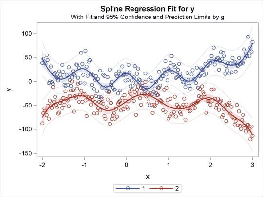
One application of ordinary multiple regression is fitting two or more regression lines through a single scatter plot. With
PROC TRANSREG, this application can easily be generalized to fit separate or parallel curves. To illustrate, consider a data
set with two groups and a group membership variable g that has the value 1 for one group and 2 for the other group. The data set also has a continuous independent variable x and a continuous dependent variable y. When g is crossed with x, the variables g1x and g2x both have a large partition of zeros. For this reason, the KNOTS= t-option is specified instead of the NKNOTS= t-option. (The latter would put a number of knots in the partition of zeros.) The following example generates an artificial data set
with two curves. While these artificial data are clearly not realistic, their distinct pattern helps illustrate how fitting
simultaneous regression functions works. The following statements generate data and show how PROC TRANSREG fits lines, curves,
and monotone curves through a scatter plot:
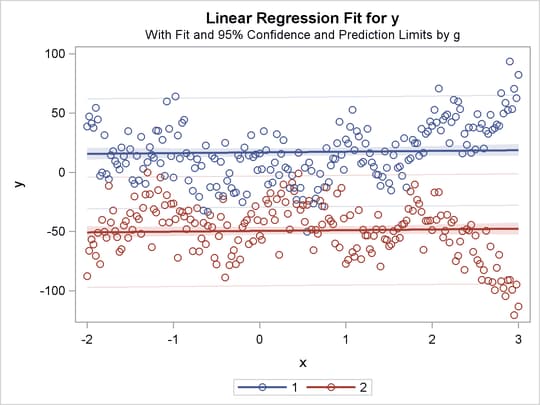
title 'Separate Curves, Separate Intercepts';
data a;
do x = -2 to 3 by 0.025;
g = 1;
y = 8*(x*x + 2*cos(x*6)) + 15*normal(7654321);
output;
g = 2;
y = 4*(-x*x + 4*sin(x*4)) - 40 + 15*normal(7654321);
output;
end;
run;
ods graphics on;
ods select fitplot(persist);
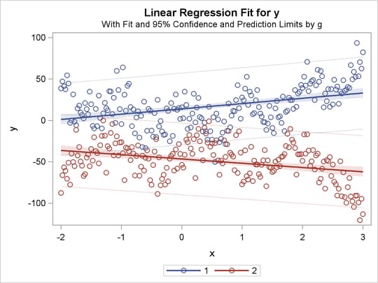
title 'Parallel Lines, Separate Intercepts';
proc transreg data=a solve;
model identity(y)=class(g) identity(x);
run;
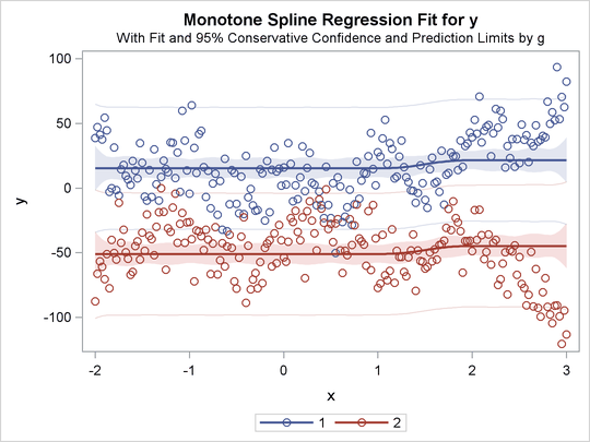
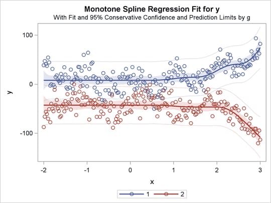
title 'Parallel Monotone Curves, Separate Intercepts';
proc transreg data=a;
model identity(y)=class(g) mspline(x / knots=-1.5 to 2.5 by 0.5);
run;
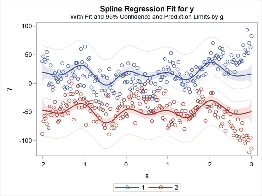
title 'Parallel Curves, Separate Intercepts';
proc transreg data=a solve;
model identity(y)=class(g) spline(x / knots=-1.5 to 2.5 by 0.5);
run;
title 'Separate Slopes, Same Intercept';
proc transreg data=a;
model identity(y)=class(g / zero=none) * identity(x);
run;
title 'Separate Monotone Curves, Same Intercept';
proc transreg data=a;
model identity(y) = class(g / zero=none) *
mspline(x / knots=-1.5 to 2.5 by 0.5);
run;
title 'Separate Curves, Same Intercept';
proc transreg data=a solve;
model identity(y) = class(g / zero=none) *
spline(x / knots=-1.5 to 2.5 by 0.5);
run;
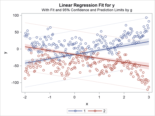
title 'Separate Slopes, Separate Intercepts';
proc transreg data=a;
model identity(y) = class(g / zero=none) | identity(x);
run;
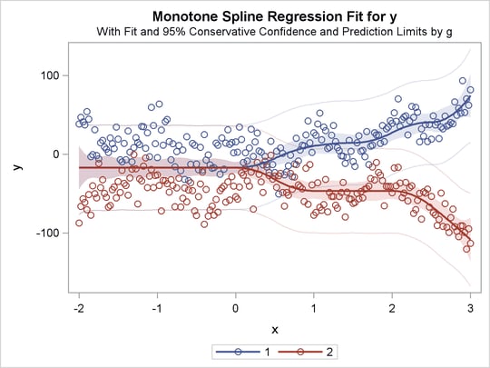
title 'Separate Monotone Curves, Separate Intercepts';
proc transreg data=a;
model identity(y) = class(g / zero=none) |
mspline(x / knots=-1.5 to 2.5 by 0.5);
run;
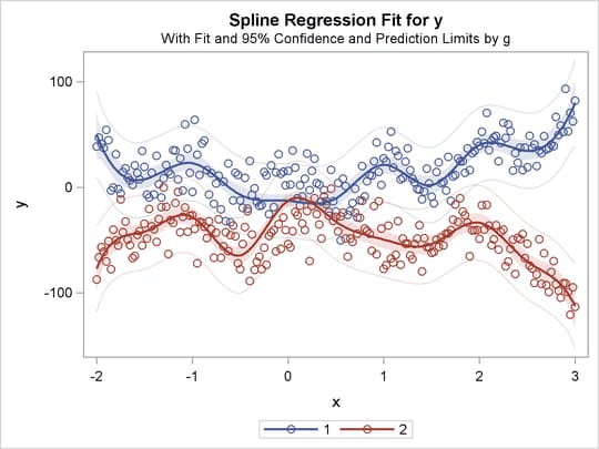
title 'Separate Curves, Separate Intercepts';
proc transreg data=a solve;
model identity(y) = class(g / zero=none) |
spline(x / knots=-1.5 to 2.5 by 0.5);
run;
ods select all;
The previous statements produce Figure 101.32 through Figure 101.40. Only the fit plots are generated and displayed.