The TRANSREG Procedure
- Overview
-
Getting Started

-
Syntax
-
DetailsModel Statement UsageBox-Cox TransformationsUsing Splines and KnotsScoring Spline VariablesLinear and Nonlinear Regression FunctionsSimultaneously Fitting Two Regression FunctionsPenalized B-SplinesSmoothing SplinesSmoothing Splines Changes and EnhancementsIteration History Changes and EnhancementsANOVA CodingsMissing ValuesMissing Values, UNTIE, and Hypothesis TestsControlling the Number of IterationsUsing the REITERATE Algorithm OptionAvoiding Constant TransformationsConstant VariablesCharacter OPSCORE VariablesConvergence and DegeneraciesImplicit and Explicit InterceptsPassive ObservationsPoint ModelsRedundancy AnalysisOptimal ScalingOPSCORE, MONOTONE, UNTIE, and LINEAR TransformationsSPLINE and MSPLINE TransformationsSpecifying the Number of KnotsSPLINE, BSPLINE, and PSPLINE ComparisonsHypothesis TestsOutput Data SetOUTTEST= Output Data SetComputational ResourcesUnbalanced ANOVA without CLASS VariablesHypothesis Tests for Simple Univariate ModelsHypothesis Tests with Monotonicity ConstraintsHypothesis Tests with Dependent Variable TransformationsHypothesis Tests with One-Way ANOVAUsing the DESIGN Output OptionDiscrete Choice Experiments: DESIGN, NORESTORE, NOZEROCenteringDisplayed OutputODS Table NamesODS Graphics
-
Examples
- References
This section illustrates some properties of splines. Splines are curves, and they are usually required to be continuous and smooth. Splines are usually defined as piecewise polynomials of degree n with function values and first n – 1 derivatives that agree at the points where they join. The abscissa or X-axis values of the join points are called knots. The term “spline” is also used for polynomials (splines with no knots) and piecewise polynomials with more than one discontinuous derivative. Splines with no knots are generally smoother than splines with knots, which are generally smoother than splines with multiple discontinuous derivatives. Splines with few knots are generally smoother than splines with many knots; however, increasing the number of knots usually increases the fit of the spline function to the data. Knots give the curve freedom to bend to more closely follow the data. See Smith (1979) for an excellent introduction to splines.
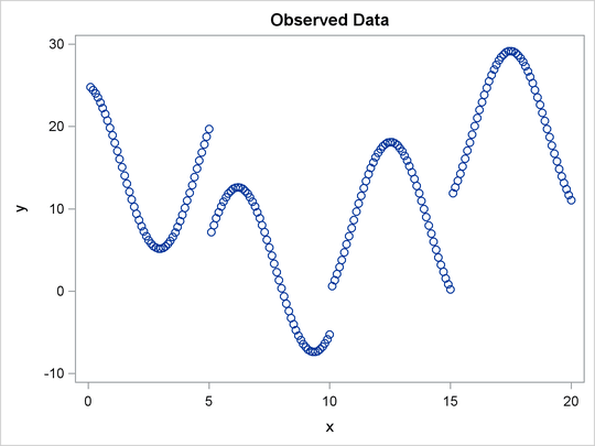
In this section, an artificial data set is created with a variable y that is a discontinuous function of x. (See Figure 101.20.) Notice that the function has four unconnected parts, each of which is a curve. Notice too that there is an overall quadratic
trend—that is, ignoring the shapes of the individual curves, at first the y values tend to decrease as x increases, then y values tend to increase. While these artificial data are clearly not realistic, their distinct pattern helps illustrate how
splines work. The following statements create the data set, fit a simple linear regression model, and produce Figure 101.19 through Figure 101.20:
title 'An Illustration of Splines and Knots';
* Create in y a discontinuous function of x.;
data a;
x = -0.000001;
do i = 0 to 199;
if mod(i, 50) = 0 then do;
c = ((x / 2) - 5)**2;
if i = 150 then c = c + 5;
y = c;
end;
x = x + 0.1;
y = y - sin(x - c);
output;
end;
run;
ods graphics on;
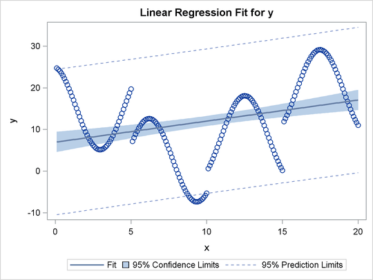
title2 'A Linear Regression Fit';
proc transreg data=a plots=scatter rsquare;
model identity(y) = identity(x);
run;
The R square for the linear regression is 0.1006. The linear fit results in Figure 101.19 show the predicted values of y given x. It can clearly be seen in Figure 101.19 that the linear regression model is not appropriate for these data.
Figure 101.19: A Linear Regression Fit
| An Illustration of Splines and Knots |
| A Linear Regression Fit |
| The TRANSREG Procedure Hypothesis Tests for Identity(y) |
| R-Square | 0.1006 |
|---|
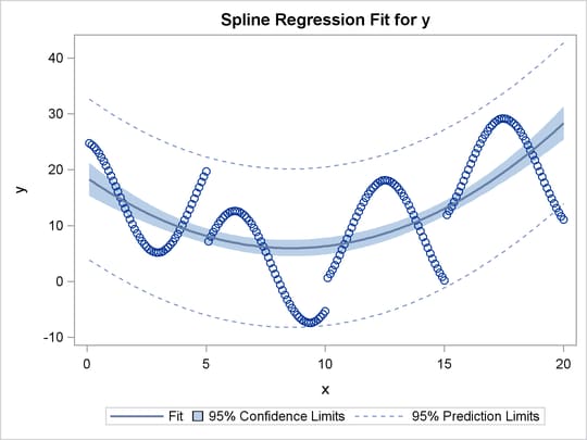
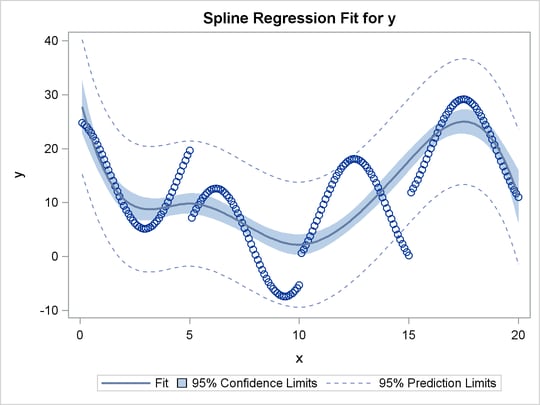
The next PROC TRANSREG step finds a degree-two spline transformation with no knots, which is a quadratic polynomial. The spline is a weighted sum of a single constant, a single straight line, and a single quadratic curve. The following statements perform the quadratic analysis and produce Figure 101.21:
title2 'A Quadratic Polynomial Fit';

proc transreg data=A;
   model identity(y)=spline(x / degree=2);
run;
The R square in Figure 101.21 increases from 0.10061, which is the linear fit value from before, to 0.40720. The plot shows that the quadratic regression function does not fit any of the individual curves well, but it does follow the overall trend in the data. Since the overall trend is quadratic, if you were to fit a degree-three spline with no knots (not shown) would increase R square by only a small amount.
Figure 101.21: A Quadratic Polynomial Fit
| An Illustration of Splines and Knots |
| A Quadratic Polynomial Fit |
| TRANSREG MORALS Algorithm Iteration History for Identity(y) | |||||
|---|---|---|---|---|---|
| Iteration Number |
Average Change |
Maximum Change |
R-Square | Criterion Change |
Note |
| 1 | 0.82127 | 2.77121 | 0.10061 | ||
| 2 | 0.00000 | 0.00000 | 0.40720 | 0.30659 | Converged |
| Algorithm converged. |
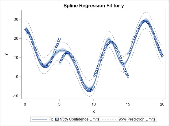
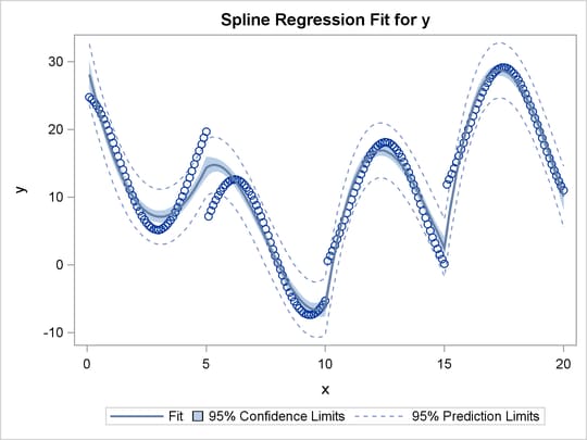
The next step uses the default degree of three, for a piecewise cubic polynomial, and requests knots at the known break points,
x=5, 10, and 15. This requests a spline that is continuous, has continuous first and second derivatives, and has a third derivative
that is discontinuous at 5, 10, and 15. The spline is a weighted sum of a single constant, a single straight line, a single
quadratic curve, a cubic curve for the portion of x less than 5, a different cubic curve for the portion of x between 5 and 10, a different cubic curve for the portion of x between 10 and 15, and another cubic curve for the portion of x greater than 15. The following statements fit the spline model and produce Figure 101.22:
title2 'A Cubic Spline Fit with Knots at X=5, 10, 15';

proc transreg data=a;
   model identity(y) = spline(x / knots=5 10 15);
run;
The new R square in Figure 101.22 is 0.61730. The plot shows that the spline is less smooth than the quadratic polynomial and follows the data more closely than the quadratic polynomial.
Figure 101.22: A Cubic Spline Fit
| An Illustration of Splines and Knots |
| A Cubic Spline Fit with Knots at X=5, 10, 15 |
| TRANSREG MORALS Algorithm Iteration History for Identity(y) | |||||
|---|---|---|---|---|---|
| Iteration Number |
Average Change |
Maximum Change |
R-Square | Criterion Change |
Note |
| 1 | 0.85367 | 3.88449 | 0.10061 | ||
| 2 | 0.00000 | 0.00000 | 0.61730 | 0.51670 | Converged |
| Algorithm converged. |
The same model could be fit with a DATA step and PROC REG, as follows:
data b;             /* A is the data set used by transreg */
   set a(keep=x y);
   x1=x;                       /* x                       */
   x2=x**2;                    /* x squared               */
   x3=x**3;                    /* x cubed                 */
   x4=(x> 5)*((x-5)**3);       /* change in x**3 after  5 */
   x5=(x>10)*((x-10)**3);      /* change in x**3 after 10 */
   x6=(x>15)*((x-15)**3);      /* change in x**3 after 15 */
run;

proc reg;
   model y=x1-x6;
run; quit;
The output from these previous statements is not displayed. The assignment statements and comments show how you can construct terms that can be used to fit the same model.
In the next step, each knot is repeated three times, so the first, second, and third derivatives are discontinuous at x=5, 10, and 15, but the spline is continuous at the knots. The spline is a weighted sum of the following:
-
a single constant
-
a line for the portion of
xless than 5 -
a quadratic curve for the portion of
xless than 5 -
a cubic curve for the portion of
xless than 5 -
a different line for the portion of
xbetween 5 and 10 -
a different quadratic curve for the portion of
xbetween 5 and 10 -
a different cubic curve for the portion of
xbetween 5 and 10 -
a different line for the portion of
xbetween 10 and 15 -
a different quadratic curve for the portion of
xbetween 10 and 15 -
a different cubic curve for the portion of
xbetween 10 and 15 -
another line for the portion of
xgreater than 15 -
another quadratic curve for the portion of
xgreater than 15 -
another cubic curve for the portion of
xgreater than 15
The spline is continuous since there is not a separate constant or separate intercept in the formula for the spline for each knot. The following statements perform this analysis and produce Figure 101.23:
title3 'First - Third Derivatives Discontinuous at X=5, 10, 15';

proc transreg data=a;
   model identity(y) = spline(x / knots=5 5 5 10 10 10 15 15 15);
run;
Now the R square in Figure 101.23 is 0.95542, and the spline closely follows the data, except at the knots.
Figure 101.23: Spline with Discontinuous Derivatives
| An Illustration of Splines and Knots |
| A Cubic Spline Fit with Knots at X=5, 10, 15 |
| First - Third Derivatives Discontinuous at X=5, 10, 15 |
| TRANSREG MORALS Algorithm Iteration History for Identity(y) | |||||
|---|---|---|---|---|---|
| Iteration Number |
Average Change |
Maximum Change |
R-Square | Criterion Change |
Note |
| 1 | 0.92492 | 3.50038 | 0.10061 | ||
| 2 | 0.00000 | 0.00000 | 0.95542 | 0.85481 | Converged |
| Algorithm converged. |
The same model could be fit with a DATA step and PROC REG, as follows:
data b;
   set a(keep=x y);
   x1=x;                        /* x                       */
   x2=x**2;                     /* x squared               */
   x3=x**3;                     /* x cubed                 */
   x4=(x>5)   * (x- 5);         /* change in x    after  5 */
   x5=(x>10)  * (x-10);         /* change in x    after 10 */
   x6=(x>15)  * (x-15);         /* change in x    after 15 */
   x7=(x>5)   * ((x-5)**2);     /* change in x**2 after  5 */
   x8=(x>10)  * ((x-10)**2);    /* change in x**2 after 10 */
   x9=(x>15)  * ((x-15)**2);    /* change in x**2 after 15 */
   x10=(x>5)  * ((x-5)**3);     /* change in x**3 after  5 */
   x11=(x>10) * ((x-10)**3);    /* change in x**3 after 10 */
   x12=(x>15) * ((x-15)**3);    /* change in x**3 after 15 */
run;

proc reg;
   model y=x1-x12;
run; quit;
The output from these previous statements is not displayed. The assignment statements and comments show how you can construct terms that can be used to fit the same model.
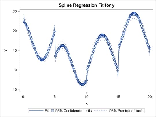
Each knot is repeated four times in the next step. Now the spline function is discontinuous at the knots, and it can follow the data more closely. The following statements perform this analysis and produce Figure 101.24:
title3 'Discontinuous Function and Derivatives';

proc transreg data=a;
   model identity(y) = spline(x / knots=5 5 5 5 10 10 10 10
                                        15 15 15 15);
run;
Now the R square in Figure 101.24 is 0.99254. In this step, each separate curve is approximated by a cubic polynomial (with no knots within the separate polynomials). (Note, however, that the separate functions are connected in the plot, because PROC TRANSREG cannot currently produce separate functions for a model like this. Usually, you would use a CLASS variable to get separate functions.)
Figure 101.24: Discontinuous Spline Fit
| An Illustration of Splines and Knots |
| A Cubic Spline Fit with Knots at X=5, 10, 15 |
| Discontinuous Function and Derivatives |
| TRANSREG MORALS Algorithm Iteration History for Identity(y) | |||||
|---|---|---|---|---|---|
| Iteration Number |
Average Change |
Maximum Change |
R-Square | Criterion Change |
Note |
| 1 | 0.90271 | 3.29184 | 0.10061 | ||
| 2 | 0.00000 | 0.00000 | 0.99254 | 0.89193 | Converged |
| Algorithm converged. |
To solve this problem with a DATA step and PROC REG, you would need to create all of the variables in the preceding DATA step
(the B data set for the piecewise polynomial with discontinuous third derivatives), plus the following three variables:
x13=(x >  5);   /* intercept change after  5 */
x14=(x > 10);   /* intercept change after 10 */
x15=(x > 15);   /* intercept change after 15 */
The next two examples use the NKNOTS= t-option to specify the number of knots but not their location. NKNOTS=4 places knots at the quintiles, whereas NKNOTS=9 places knots at the deciles. The spline and its first two derivatives are continuous. The following statements produce Figure 101.25 and Figure 101.26:
title3 'Four Knots';

proc transreg data=a;
   model identity(y) = spline(x / nknots=4);
run;

title3 'Nine Knots';

proc transreg data=a;
   model identity(y) = spline(x / nknots=9);
run;
The R-square values displayed in Figure 101.25 and Figure 101.26 are 0.74450 and 0.95256, respectively. Even though the knots are not optimally placed, the spline can closely follow the data with NKNOTS=9.
Figure 101.25: Spline Fit with Knots at the Quintiles
| An Illustration of Splines and Knots |
| A Cubic Spline Fit with Knots at X=5, 10, 15 |
| Four Knots |
| TRANSREG MORALS Algorithm Iteration History for Identity(y) | |||||
|---|---|---|---|---|---|
| Iteration Number |
Average Change |
Maximum Change |
R-Square | Criterion Change |
Note |
| 1 | 0.90305 | 4.46027 | 0.10061 | ||
| 2 | 0.00000 | 0.00000 | 0.74450 | 0.64389 | Converged |
| Algorithm converged. |
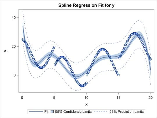
Figure 101.26: Spline Fit with Knots at the Deciles
| An Illustration of Splines and Knots |
| A Cubic Spline Fit with Knots at X=5, 10, 15 |
| Nine Knots |
| TRANSREG MORALS Algorithm Iteration History for Identity(y) | |||||
|---|---|---|---|---|---|
| Iteration Number |
Average Change |
Maximum Change |
R-Square | Criterion Change |
Note |
| 1 | 0.94832 | 3.03488 | 0.10061 | ||
| 2 | 0.00000 | 0.00000 | 0.95256 | 0.85196 | Converged |
| Algorithm converged. |