The TRANSREG Procedure
- Overview
-
Getting Started

-
Syntax
-
DetailsModel Statement UsageBox-Cox TransformationsUsing Splines and KnotsScoring Spline VariablesLinear and Nonlinear Regression FunctionsSimultaneously Fitting Two Regression FunctionsPenalized B-SplinesSmoothing SplinesSmoothing Splines Changes and EnhancementsIteration History Changes and EnhancementsANOVA CodingsMissing ValuesMissing Values, UNTIE, and Hypothesis TestsControlling the Number of IterationsUsing the REITERATE Algorithm OptionAvoiding Constant TransformationsConstant VariablesCharacter OPSCORE VariablesConvergence and DegeneraciesImplicit and Explicit InterceptsPassive ObservationsPoint ModelsRedundancy AnalysisOptimal ScalingOPSCORE, MONOTONE, UNTIE, and LINEAR TransformationsSPLINE and MSPLINE TransformationsSpecifying the Number of KnotsSPLINE, BSPLINE, and PSPLINE ComparisonsHypothesis TestsOutput Data SetOUTTEST= Output Data SetComputational ResourcesUnbalanced ANOVA without CLASS VariablesHypothesis Tests for Simple Univariate ModelsHypothesis Tests with Monotonicity ConstraintsHypothesis Tests with Dependent Variable TransformationsHypothesis Tests with One-Way ANOVAUsing the DESIGN Output OptionDiscrete Choice Experiments: DESIGN, NORESTORE, NOZEROCenteringDisplayed OutputODS Table NamesODS Graphics
-
Examples
- References
This section shows you how to find spline transformations of variables in one data set and apply the same transformations
to variables in another data set. This is illustrated with artificial data. In these data sets, the variable y is approximately a linear function of nonlinear transformations of the variables x, w, and z. The model is fit using data set X, and those results are used to score data set Z. The following statements create the two data sets:
title 'An Illustration of Splines and Knots';
title2 'Scoring Spline Variables';

data x;
   do i = 1 to 5000;
      w = normal(7);
      x = normal(7);
      z = normal(7);
      y = w * w + log(5 + x) + sin(z) + normal(7);
      output;
   end;
run;
data z;
   do i = 1 to 5000;
      w = normal(1);
      x = normal(1);
      z = normal(1);
      y = w * w + log(5 + x) + sin(z) + normal(1);
      output;
   end;
run;
First, you run PROC TRANSREG to fit the transformation regression model asking for spline transformations of the three independent
variables. You must use the EXKNOTS= t-option, because you need to use the same knots, both interior and exterior, with both data sets. By default, the exterior knots
will be different if the minima and maxima are different in the two data sets, so you get the wrong results if you do not
specify the EXKNOTS= t-option with values less than the minima and greater than the maxima of the six x, y, and w variables. If the ranges in all three pairs were different, you would need separate spline transformation for each variable
with different knot and exterior knot specifications. The following statements fit the spline model:
proc transreg data=x solve details ss2;
   ods output splinecoef=c;
   model identity(y) = spline(w x z / knots=-1.5 to 1.5 by 0.5
                                      exknots=-5 5);
   output out=d;
run;
The results of this step are not displayed. The nonprinting SplineCoef table is output to a SAS data set. This data set contains the coefficients that were used to get the spline transformations and can be used to transform variables in other data sets. These coefficients are also in the details table. However, in the SplineCoef table, they are in a form directly suitable for use with PROC SCORE.
The next step reads the second input data set, Z, and generates an output data set with the B-spline basis for each of the variables:
proc transreg data=z design;
   model bspl(w x z / knots=-1.5 to 1.5 by 0.5 exknots=-5 5);
   output out=b;
run;
Note that the same interior and exterior knots are used in both of the previous steps. The next three steps score the B-spline bases created in the previous step by using the coefficients generated in the first PROC TRANSREG step. PROC SCORE is run once for each SPLINE variable in the statements that follow:
proc score data=b score=c out=o1(rename=(spline=bw w=nw));
   var w:;
run;

proc score data=b score=c out=o2(rename=(spline=bx x=nx));
   var x:;
run;

proc score data=b score=c out=o3(rename=(spline=bz z=nz));
   var z:;
run;
The following steps merge the three transformations with the original data and plot the results:
data all;
   merge d(keep=w x z tw tx tz) o1(keep=nw bw)
         o2(keep=nx bx) o3(keep=nz bz);
run;

proc template;
   define statgraph twobytwo;
      begingraph;
         layout lattice / rows=2 columns=2;
            layout overlay;
               seriesplot y=tw x=w  / connectorder=xaxis;
               seriesplot y=bw x=nw / connectorder=xaxis;
            endlayout;
            layout overlay;
               seriesplot y=tx x=x  / connectorder=xaxis;
               seriesplot y=bx x=nx / connectorder=xaxis;
            endlayout;
            layout overlay;
               seriesplot y=tz x=z  / connectorder=xaxis;
               seriesplot y=bz x=nz / connectorder=xaxis;
            endlayout;
         endlayout;
      endgraph;
   end;
run;

proc sgrender data=all template=twobytwo;
run;
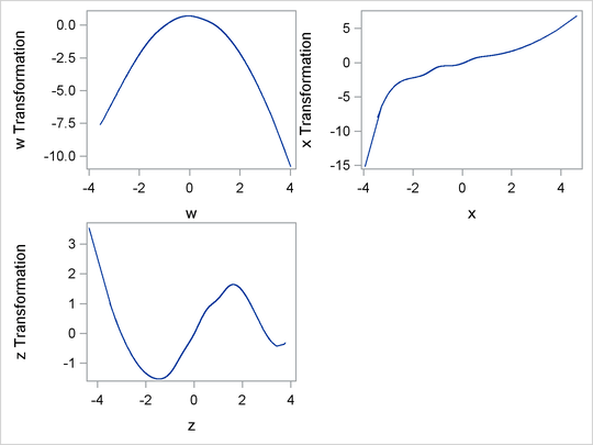
The plots in Figure 101.27 show that the two transformations for each variable, original and scored, are the same function. The two functions in each
plot are on top of each other and are indistinguishable. Furthermore, PROC TRANSREG found the functional forms that were used
to generate the data: quadratic for w, log for x, and sine for z.
The next statements show how to run PROC TRANSREG, output the interior and exterior knots to an output data set with ODS, extract the knots, and use them in a DATA step to re-create the B-spline basis that PROC TRANSREG makes. In practice, you would never need to use a DATA step to make the B-spline basis since PROC TRANSREG does it automatically. The following statements show how you could do it yourself:
data x;
   input x @@;
   datalines;
1 2 3 4 5 6 7 8 9 10
;
ods output details=d;
proc transreg details design;
   model bspline(x / nkn=3);
   output out=y;
run;
%let k = 0;
data d;
   set d;
   length d $ 20;
   retain d ' ';
   if description ne ' ' then d = description;
   if d = 'Degree' then call symput('d', compress(formattedvalue));
   if d = 'Number of Knots'
      then call symput('k', compress(formattedvalue));
   if index(d, 'Knots') and not index(d, 'Number');
   keep d numericvalue;
run;

%let nkn = %eval(&d * 2 + &k); /* total number of knots   */
%let nb  = %eval(&d + 1 + &k); /* number of cols in basis */

proc transpose data=d out=k(drop=_name_) prefix=Knot;
run;

proc print; format k: 20.16;
run;

data b(keep=x:);
   if _n_ = 1 then set k; /* read knots from transreg */
   array k[&nkn] knot1-knot&nkn;        /* knots      */
   array b[&nb] x_0 - x_%eval(&nb - 1); /* basis      */
   array w[%eval(2 * &d)];              /* work       */
   set x;
   do i = 1 to &nb; b[i] = 0; end;

   * find the index of first knot greater than current data value;
   do ki = 1 to &nkn while(k[ki] le x); end;
   kki = ki - &d - 1;

   * make the basis;
   b[1 + kki] = 1;
   do j = 1 to &d;
      w[&d + j] = k[ki + j - 1] - x;
      w[j] = x - k[ki - j];
      s = 0;
      do i = 1 to j;
         t = w[&d + i] + w[j + 1 - i];
         if t ne 0.0 then t = b[i + kki] / t;
         b[i + kki] = s + w[&d + i] * t;
         s = w[j + 1 - i] * t;
      end;
      b[j + 1 + kki] = s;
   end;
run;
proc compare data=y(keep=x:) compare=b
   criterion=1e-12 note nosummary;
   title3 "should be no differences";
run;
The output from these steps is not shown. There are several things to note about the DATA step. It produces the same basis
as PROC TRANSREG only because it uses exactly the same interior and exterior knots. The exterior knots (0.999999999999 and
10.000000000001) are just slightly smaller than 1 (the minimum in x) and just slightly greater than 10 (the maximum in x). Both exterior knots appear in the list three times, because a cubic (degree 3) polynomial was requested. The complete knot
list is: 0.999999999999 0.999999999999 0.999999999999 3 6 8 10.000000000001 10.000000000001 10.000000000001. The exterior
knots do not have any particular interpretation, but they are needed by the algorithm to construct the proper basis. The construction
method computes differences between each value and the nearby knots. The algorithm that makes the B-spline basis is not very
obvious, particularly compared to the polynomial spline basis. However, the B-spline basis is much better behaved numerically
than a polynomial-spline basis, so that is why it is used.