The TRANSREG Procedure
- Overview
-
Getting Started

-
Syntax
-
DetailsModel Statement UsageBox-Cox TransformationsUsing Splines and KnotsScoring Spline VariablesLinear and Nonlinear Regression FunctionsSimultaneously Fitting Two Regression FunctionsPenalized B-SplinesSmoothing SplinesSmoothing Splines Changes and EnhancementsIteration History Changes and EnhancementsANOVA CodingsMissing ValuesMissing Values, UNTIE, and Hypothesis TestsControlling the Number of IterationsUsing the REITERATE Algorithm OptionAvoiding Constant TransformationsConstant VariablesCharacter OPSCORE VariablesConvergence and DegeneraciesImplicit and Explicit InterceptsPassive ObservationsPoint ModelsRedundancy AnalysisOptimal ScalingOPSCORE, MONOTONE, UNTIE, and LINEAR TransformationsSPLINE and MSPLINE TransformationsSpecifying the Number of KnotsSPLINE, BSPLINE, and PSPLINE ComparisonsHypothesis TestsOutput Data SetOUTTEST= Output Data SetComputational ResourcesUnbalanced ANOVA without CLASS VariablesHypothesis Tests for Simple Univariate ModelsHypothesis Tests with Monotonicity ConstraintsHypothesis Tests with Dependent Variable TransformationsHypothesis Tests with One-Way ANOVAUsing the DESIGN Output OptionDiscrete Choice Experiments: DESIGN, NORESTORE, NOZEROCenteringDisplayed OutputODS Table NamesODS Graphics
-
Examples
- References
This section illustrates several different codings of classification variables and hence several different ways of fitting
two-way ANOVA models to some data. Each example fits an ANOVA model, displays the ANOVA table and parameter estimates, and
displays the coded design matrix. Note throughout that the ANOVA tables and R squares are identical for all of the models,
showing that the codings are equivalent. For each model, the parameter estimates are stated as a function of the cell means.
The formulas are appropriate for a design such as this one, which is balanced and orthogonal (every level and every pair of
levels occurs equally often). They will not work with unequal frequencies. Since this data set has ![]() cells, the full-rank codings all have six parameters. The following statements create the input data set, and display it
in Figure 101.43:
cells, the full-rank codings all have six parameters. The following statements create the input data set, and display it
in Figure 101.43:
title 'Two-Way ANOVA Models';

data x;
   input a b @@;
   do i = 1 to 2; input y @@; output; end;
   drop i;
   datalines;
1 1   16 14         1 2   15 13
2 1    1  9         2 2   12 20
3 1   14  8         3 2   18 20
;
proc print label;
run;
Figure 101.43: Input Data Set
| Two-Way ANOVA Models |
| Obs | a | b | y |
|---|---|---|---|
| 1 | 1 | 1 | 16 |
| 2 | 1 | 1 | 14 |
| 3 | 1 | 2 | 15 |
| 4 | 1 | 2 | 13 |
| 5 | 2 | 1 | 1 |
| 6 | 2 | 1 | 9 |
| 7 | 2 | 2 | 12 |
| 8 | 2 | 2 | 20 |
| 9 | 3 | 1 | 14 |
| 10 | 3 | 1 | 8 |
| 11 | 3 | 2 | 18 |
| 12 | 3 | 2 | 20 |
The following statements fit a cell-means model and produce Figure 101.44 and Figure 101.45:
proc transreg data=x ss2 short;
   title2 'Cell-Means Model';
   model identity(y) = class(a * b / zero=none);
   output replace;
run;

proc print label;
run;
Figure 101.44: Cell-Means Model
| Two-Way ANOVA Models |
| Cell-Means Model |
| Dependent Variable Identity(y) |
| Class Level Information | ||
|---|---|---|
| Class | Levels | Values |
| a | 3 | 1 2 3 |
| b | 2 | 1 2 |
| Number of Observations Read | 12 |
|---|---|
| Number of Observations Used | 12 |
| Implicit Intercept Model |
| The TRANSREG Procedure Hypothesis Tests for Identity(y) |
| Univariate ANOVA Table Based on the Usual Degrees of Freedom | |||||
|---|---|---|---|---|---|
| Source | DF | Sum of Squares | Mean Square | F Value | Pr > F |
| Model | 5 | 234.6667 | 46.93333 | 3.20 | 0.0946 |
| Error | 6 | 88.0000 | 14.66667 | ||
| Corrected Total | 11 | 322.6667 | |||
| Root MSE | 3.82971 | R-Square | 0.7273 |
|---|---|---|---|
| Dependent Mean | 13.33333 | Adj R-Sq | 0.5000 |
| Coeff Var | 28.72281 |
| Univariate Regression Table Based on the Usual Degrees of Freedom | |||||||
|---|---|---|---|---|---|---|---|
| Variable | DF | Coefficient | Type II Sum of Squares |
Mean Square | F Value | Pr > F | Label |
| Class.a1b1 | 1 | 15.0000000 | 450.000 | 450.000 | 30.68 | 0.0015 | a 1 * b 1 |
| Class.a1b2 | 1 | 14.0000000 | 392.000 | 392.000 | 26.73 | 0.0021 | a 1 * b 2 |
| Class.a2b1 | 1 | 5.0000000 | 50.000 | 50.000 | 3.41 | 0.1144 | a 2 * b 1 |
| Class.a2b2 | 1 | 16.0000000 | 512.000 | 512.000 | 34.91 | 0.0010 | a 2 * b 2 |
| Class.a3b1 | 1 | 11.0000000 | 242.000 | 242.000 | 16.50 | 0.0066 | a 3 * b 1 |
| Class.a3b2 | 1 | 19.0000000 | 722.000 | 722.000 | 49.23 | 0.0004 | a 3 * b 2 |
The parameter estimates are
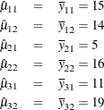
Figure 101.45: Cell-Means Model, Design Matrix
| Two-Way ANOVA Models |
| Cell-Means Model |
| Obs | _TYPE_ | _NAME_ | y | Intercept | a 1 * b 1 |
a 1 * b 2 |
a 2 * b 1 |
a 2 * b 2 |
a 3 * b 1 |
a 3 * b 2 |
a | b |
|---|---|---|---|---|---|---|---|---|---|---|---|---|
| 1 | SCORE | ROW1 | 16 | . | 1 | 0 | 0 | 0 | 0 | 0 | 1 | 1 |
| 2 | SCORE | ROW2 | 14 | . | 1 | 0 | 0 | 0 | 0 | 0 | 1 | 1 |
| 3 | SCORE | ROW3 | 15 | . | 0 | 1 | 0 | 0 | 0 | 0 | 1 | 2 |
| 4 | SCORE | ROW4 | 13 | . | 0 | 1 | 0 | 0 | 0 | 0 | 1 | 2 |
| 5 | SCORE | ROW5 | 1 | . | 0 | 0 | 1 | 0 | 0 | 0 | 2 | 1 |
| 6 | SCORE | ROW6 | 9 | . | 0 | 0 | 1 | 0 | 0 | 0 | 2 | 1 |
| 7 | SCORE | ROW7 | 12 | . | 0 | 0 | 0 | 1 | 0 | 0 | 2 | 2 |
| 8 | SCORE | ROW8 | 20 | . | 0 | 0 | 0 | 1 | 0 | 0 | 2 | 2 |
| 9 | SCORE | ROW9 | 14 | . | 0 | 0 | 0 | 0 | 1 | 0 | 3 | 1 |
| 10 | SCORE | ROW10 | 8 | . | 0 | 0 | 0 | 0 | 1 | 0 | 3 | 1 |
| 11 | SCORE | ROW11 | 18 | . | 0 | 0 | 0 | 0 | 0 | 1 | 3 | 2 |
| 12 | SCORE | ROW12 | 20 | . | 0 | 0 | 0 | 0 | 0 | 1 | 3 | 2 |
The next model is a reference cell model, and the default reference cell is the last cell, which in this case is the (3,2) cell. The following statements fit a reference cell model and produce Figure 101.46 and Figure 101.47:
proc transreg data=x ss2 short;
   title2 'Reference Cell Model, (3,2) Reference Cell';
   model identity(y) = class(a | b);
   output replace;
run;

proc print label;
run;
Figure 101.46: Reference Cell Model, (3,2) Reference Cell
| Two-Way ANOVA Models |
| Reference Cell Model, (3,2) Reference Cell |
| Dependent Variable Identity(y) |
| Class Level Information | ||
|---|---|---|
| Class | Levels | Values |
| a | 3 | 1 2 3 |
| b | 2 | 1 2 |
| Number of Observations Read | 12 |
|---|---|
| Number of Observations Used | 12 |
| The TRANSREG Procedure Hypothesis Tests for Identity(y) |
| Univariate ANOVA Table Based on the Usual Degrees of Freedom | |||||
|---|---|---|---|---|---|
| Source | DF | Sum of Squares | Mean Square | F Value | Pr > F |
| Model | 5 | 234.6667 | 46.93333 | 3.20 | 0.0946 |
| Error | 6 | 88.0000 | 14.66667 | ||
| Corrected Total | 11 | 322.6667 | |||
| Root MSE | 3.82971 | R-Square | 0.7273 |
|---|---|---|---|
| Dependent Mean | 13.33333 | Adj R-Sq | 0.5000 |
| Coeff Var | 28.72281 |
| Univariate Regression Table Based on the Usual Degrees of Freedom | |||||||
|---|---|---|---|---|---|---|---|
| Variable | DF | Coefficient | Type II Sum of Squares |
Mean Square | F Value | Pr > F | Label |
| Intercept | 1 | 19.0000000 | 722.000 | 722.000 | 49.23 | 0.0004 | Intercept |
| Class.a1 | 1 | -5.0000000 | 25.000 | 25.000 | 1.70 | 0.2395 | a 1 |
| Class.a2 | 1 | -3.0000000 | 9.000 | 9.000 | 0.61 | 0.4632 | a 2 |
| Class.b1 | 1 | -8.0000000 | 64.000 | 64.000 | 4.36 | 0.0817 | b 1 |
| Class.a1b1 | 1 | 9.0000000 | 40.500 | 40.500 | 2.76 | 0.1476 | a 1 * b 1 |
| Class.a2b1 | 1 | -3.0000000 | 4.500 | 4.500 | 0.31 | 0.5997 | a 2 * b 1 |
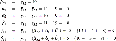
Figure 101.47: Reference Cell Model, (3,2) Reference Cell, Design Matrix
| Two-Way ANOVA Models |
| Reference Cell Model, (3,2) Reference Cell |
| Obs | _TYPE_ | _NAME_ | y | Intercept | a 1 | a 2 | b 1 | a 1 * b 1 |
a 2 * b 1 |
a | b |
|---|---|---|---|---|---|---|---|---|---|---|---|
| 1 | SCORE | ROW1 | 16 | 1 | 1 | 0 | 1 | 1 | 0 | 1 | 1 |
| 2 | SCORE | ROW2 | 14 | 1 | 1 | 0 | 1 | 1 | 0 | 1 | 1 |
| 3 | SCORE | ROW3 | 15 | 1 | 1 | 0 | 0 | 0 | 0 | 1 | 2 |
| 4 | SCORE | ROW4 | 13 | 1 | 1 | 0 | 0 | 0 | 0 | 1 | 2 |
| 5 | SCORE | ROW5 | 1 | 1 | 0 | 1 | 1 | 0 | 1 | 2 | 1 |
| 6 | SCORE | ROW6 | 9 | 1 | 0 | 1 | 1 | 0 | 1 | 2 | 1 |
| 7 | SCORE | ROW7 | 12 | 1 | 0 | 1 | 0 | 0 | 0 | 2 | 2 |
| 8 | SCORE | ROW8 | 20 | 1 | 0 | 1 | 0 | 0 | 0 | 2 | 2 |
| 9 | SCORE | ROW9 | 14 | 1 | 0 | 0 | 1 | 0 | 0 | 3 | 1 |
| 10 | SCORE | ROW10 | 8 | 1 | 0 | 0 | 1 | 0 | 0 | 3 | 1 |
| 11 | SCORE | ROW11 | 18 | 1 | 0 | 0 | 0 | 0 | 0 | 3 | 2 |
| 12 | SCORE | ROW12 | 20 | 1 | 0 | 0 | 0 | 0 | 0 | 3 | 2 |
The next model is a deviations-from-means model. This coding is also called effects coding. The default reference cell is the last cell (3,2). The following statements produce Figure 101.48 and Figure 101.49:
proc transreg data=x ss2 short;
   title2 'Deviations from Means, (3,2) Reference Cell';
   model identity(y) = class(a | b / deviations);
   output replace;
run;

proc print label;
run;
Figure 101.48: Deviations-from-Means Model, (3,2) Reference Cell
| Two-Way ANOVA Models |
| Deviations from Means, (3,2) Reference Cell |
| Dependent Variable Identity(y) |
| Class Level Information | ||
|---|---|---|
| Class | Levels | Values |
| a | 3 | 1 2 3 |
| b | 2 | 1 2 |
| Number of Observations Read | 12 |
|---|---|
| Number of Observations Used | 12 |
| The TRANSREG Procedure Hypothesis Tests for Identity(y) |
| Univariate ANOVA Table Based on the Usual Degrees of Freedom | |||||
|---|---|---|---|---|---|
| Source | DF | Sum of Squares | Mean Square | F Value | Pr > F |
| Model | 5 | 234.6667 | 46.93333 | 3.20 | 0.0946 |
| Error | 6 | 88.0000 | 14.66667 | ||
| Corrected Total | 11 | 322.6667 | |||
| Root MSE | 3.82971 | R-Square | 0.7273 |
|---|---|---|---|
| Dependent Mean | 13.33333 | Adj R-Sq | 0.5000 |
| Coeff Var | 28.72281 |
| Univariate Regression Table Based on the Usual Degrees of Freedom | |||||||
|---|---|---|---|---|---|---|---|
| Variable | DF | Coefficient | Type II Sum of Squares |
Mean Square | F Value | Pr > F | Label |
| Intercept | 1 | 13.3333333 | 2133.33 | 2133.33 | 145.45 | <.0001 | Intercept |
| Class.a1 | 1 | 1.1666667 | 8.17 | 8.17 | 0.56 | 0.4837 | a 1 |
| Class.a2 | 1 | -2.8333333 | 48.17 | 48.17 | 3.28 | 0.1199 | a 2 |
| Class.b1 | 1 | -3.0000000 | 108.00 | 108.00 | 7.36 | 0.0349 | b 1 |
| Class.a1b1 | 1 | 3.5000000 | 73.50 | 73.50 | 5.01 | 0.0665 | a 1 * b 1 |
| Class.a2b1 | 1 | -2.5000000 | 37.50 | 37.50 | 2.56 | 0.1609 | a 2 * b 1 |
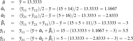
Figure 101.49: Deviations-from-Means Model, (3,2) Reference Cell, Design Matrix
| Two-Way ANOVA Models |
| Deviations from Means, (3,2) Reference Cell |
| Obs | _TYPE_ | _NAME_ | y | Intercept | a 1 | a 2 | b 1 | a 1 * b 1 | a 2 * b 1 | a | b |
|---|---|---|---|---|---|---|---|---|---|---|---|
| 1 | SCORE | ROW1 | 16 | 1 | 1 | 0 | 1 | 1 | 0 | 1 | 1 |
| 2 | SCORE | ROW2 | 14 | 1 | 1 | 0 | 1 | 1 | 0 | 1 | 1 |
| 3 | SCORE | ROW3 | 15 | 1 | 1 | 0 | -1 | -1 | 0 | 1 | 2 |
| 4 | SCORE | ROW4 | 13 | 1 | 1 | 0 | -1 | -1 | 0 | 1 | 2 |
| 5 | SCORE | ROW5 | 1 | 1 | 0 | 1 | 1 | 0 | 1 | 2 | 1 |
| 6 | SCORE | ROW6 | 9 | 1 | 0 | 1 | 1 | 0 | 1 | 2 | 1 |
| 7 | SCORE | ROW7 | 12 | 1 | 0 | 1 | -1 | 0 | -1 | 2 | 2 |
| 8 | SCORE | ROW8 | 20 | 1 | 0 | 1 | -1 | 0 | -1 | 2 | 2 |
| 9 | SCORE | ROW9 | 14 | 1 | -1 | -1 | 1 | -1 | -1 | 3 | 1 |
| 10 | SCORE | ROW10 | 8 | 1 | -1 | -1 | 1 | -1 | -1 | 3 | 1 |
| 11 | SCORE | ROW11 | 18 | 1 | -1 | -1 | -1 | 1 | 1 | 3 | 2 |
| 12 | SCORE | ROW12 | 20 | 1 | -1 | -1 | -1 | 1 | 1 | 3 | 2 |
The next model is a less-than-full-rank model. The parameter estimates are constrained to sum to zero within each effect. The following statements produce Figure 101.50 and Figure 101.51:
proc transreg data=x ss2 short;
   title2 'Less-Than-Full-Rank Model';
   model identity(y) = class(a | b / zero=sum);
   output replace;
run;

proc print label;
run;
Figure 101.50: Less-Than-Full-Rank Model
| Two-Way ANOVA Models |
| Less-Than-Full-Rank Model |
| Dependent Variable Identity(y) |
| Class Level Information | ||
|---|---|---|
| Class | Levels | Values |
| a | 3 | 1 2 3 |
| b | 2 | 1 2 |
| Number of Observations Read | 12 |
|---|---|
| Number of Observations Used | 12 |
| The TRANSREG Procedure Hypothesis Tests for Identity(y) |
| Univariate ANOVA Table Based on the Usual Degrees of Freedom | |||||
|---|---|---|---|---|---|
| Source | DF | Sum of Squares | Mean Square | F Value | Pr > F |
| Model | 5 | 234.6667 | 46.93333 | 3.20 | 0.0946 |
| Error | 6 | 88.0000 | 14.66667 | ||
| Corrected Total | 11 | 322.6667 | |||
| Root MSE | 3.82971 | R-Square | 0.7273 |
|---|---|---|---|
| Dependent Mean | 13.33333 | Adj R-Sq | 0.5000 |
| Coeff Var | 28.72281 |
| Univariate Regression Table Based on the Usual Degrees of Freedom | |||||||
|---|---|---|---|---|---|---|---|
| Variable | DF | Coefficient | Type II Sum of Squares |
Mean Square | F Value | Pr > F | Label |
| Intercept | 1 | 13.3333333 | 2133.33 | 2133.33 | 145.45 | <.0001 | Intercept |
| Class.a1 | 1 | 1.1666667 | 8.17 | 8.17 | 0.56 | 0.4837 | a 1 |
| Class.a2 | 1 | -2.8333333 | 48.17 | 48.17 | 3.28 | 0.1199 | a 2 |
| Class.a3 | 1 | 1.6666667 | 16.67 | 16.67 | 1.14 | 0.3274 | a 3 |
| Class.b1 | 1 | -3.0000000 | 108.00 | 108.00 | 7.36 | 0.0349 | b 1 |
| Class.b2 | 1 | 3.0000000 | 108.00 | 108.00 | 7.36 | 0.0349 | b 2 |
| Class.a1b1 | 1 | 3.5000000 | 73.50 | 73.50 | 5.01 | 0.0665 | a 1 * b 1 |
| Class.a1b2 | 1 | -3.5000000 | 73.50 | 73.50 | 5.01 | 0.0665 | a 1 * b 2 |
| Class.a2b1 | 1 | -2.5000000 | 37.50 | 37.50 | 2.56 | 0.1609 | a 2 * b 1 |
| Class.a2b2 | 1 | 2.5000000 | 37.50 | 37.50 | 2.56 | 0.1609 | a 2 * b 2 |
| Class.a3b1 | 1 | -1.0000000 | 6.00 | 6.00 | 0.41 | 0.5461 | a 3 * b 1 |
| Class.a3b2 | 1 | 1.0000000 | 6.00 | 6.00 | 0.41 | 0.5461 | a 3 * b 2 |
| The sum of the regression table DF's, minus one for the intercept, will be greater than the model df when there are ZERO=SUM constraints. |
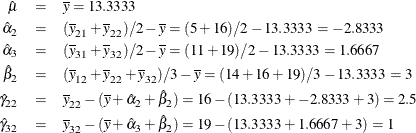
The constraints are
Only four of the five interaction constraints are needed. The fifth constraint is implied by the other four. (Given a ![]() table with four marginal sum-to-zero constraints, you can freely fill in only two cells. The values in the other four cells
are determined from the first two cells and the constraints.) A full-rank model has six estimable parameters. This less-than-full-rank
model has one parameter for the intercept, two for the first main effect (plus one more as determined by the first constraint),
one for the second main effect (plus one more as determined by the second constraint), and two for the interactions (plus
four more as determined by the next four constraints). Six of the twelve parameters are determined given the other six and
the constraints. Notice that
table with four marginal sum-to-zero constraints, you can freely fill in only two cells. The values in the other four cells
are determined from the first two cells and the constraints.) A full-rank model has six estimable parameters. This less-than-full-rank
model has one parameter for the intercept, two for the first main effect (plus one more as determined by the first constraint),
one for the second main effect (plus one more as determined by the second constraint), and two for the interactions (plus
four more as determined by the next four constraints). Six of the twelve parameters are determined given the other six and
the constraints. Notice that ![]() and
and ![]() match the corresponding estimates from the effects coding.
match the corresponding estimates from the effects coding.
Figure 101.51: Less-Than-Full-Rank Model, Design Matrix
| Two-Way ANOVA Models |
| Less-Than-Full-Rank Model |
| Obs | _TYPE_ | _NAME_ | y | Intercept | a 1 | a 2 | a 3 | b 1 | b 2 | a 1 * b 1 |
a 1 * b 2 |
a 2 * b 1 |
a 2 * b 2 |
a 3 * b 1 |
a 3 * b 2 |
a | b |
|---|---|---|---|---|---|---|---|---|---|---|---|---|---|---|---|---|---|
| 1 | SCORE | ROW1 | 16 | 1 | 1 | 0 | 0 | 1 | 0 | 1 | 0 | 0 | 0 | 0 | 0 | 1 | 1 |
| 2 | SCORE | ROW2 | 14 | 1 | 1 | 0 | 0 | 1 | 0 | 1 | 0 | 0 | 0 | 0 | 0 | 1 | 1 |
| 3 | SCORE | ROW3 | 15 | 1 | 1 | 0 | 0 | 0 | 1 | 0 | 1 | 0 | 0 | 0 | 0 | 1 | 2 |
| 4 | SCORE | ROW4 | 13 | 1 | 1 | 0 | 0 | 0 | 1 | 0 | 1 | 0 | 0 | 0 | 0 | 1 | 2 |
| 5 | SCORE | ROW5 | 1 | 1 | 0 | 1 | 0 | 1 | 0 | 0 | 0 | 1 | 0 | 0 | 0 | 2 | 1 |
| 6 | SCORE | ROW6 | 9 | 1 | 0 | 1 | 0 | 1 | 0 | 0 | 0 | 1 | 0 | 0 | 0 | 2 | 1 |
| 7 | SCORE | ROW7 | 12 | 1 | 0 | 1 | 0 | 0 | 1 | 0 | 0 | 0 | 1 | 0 | 0 | 2 | 2 |
| 8 | SCORE | ROW8 | 20 | 1 | 0 | 1 | 0 | 0 | 1 | 0 | 0 | 0 | 1 | 0 | 0 | 2 | 2 |
| 9 | SCORE | ROW9 | 14 | 1 | 0 | 0 | 1 | 1 | 0 | 0 | 0 | 0 | 0 | 1 | 0 | 3 | 1 |
| 10 | SCORE | ROW10 | 8 | 1 | 0 | 0 | 1 | 1 | 0 | 0 | 0 | 0 | 0 | 1 | 0 | 3 | 1 |
| 11 | SCORE | ROW11 | 18 | 1 | 0 | 0 | 1 | 0 | 1 | 0 | 0 | 0 | 0 | 0 | 1 | 3 | 2 |
| 12 | SCORE | ROW12 | 20 | 1 | 0 | 0 | 1 | 0 | 1 | 0 | 0 | 0 | 0 | 0 | 1 | 3 | 2 |
The next model is a reference cell model, but this time the reference cell is the first cell (1,1). The following statements produce Figure 101.52 and Figure 101.53:
proc transreg data=x ss2 short;
   title2 'Reference Cell Model, (1,1) Reference Cell';
   model identity(y) = class(a | b / zero=first);
   output replace;
run;

proc print label;
run;
Figure 101.52: Reference Cell Model, (1,1) Reference Cell
| Two-Way ANOVA Models |
| Reference Cell Model, (1,1) Reference Cell |
| Dependent Variable Identity(y) |
| Class Level Information | ||
|---|---|---|
| Class | Levels | Values |
| a | 3 | 1 2 3 |
| b | 2 | 1 2 |
| Number of Observations Read | 12 |
|---|---|
| Number of Observations Used | 12 |
| The TRANSREG Procedure Hypothesis Tests for Identity(y) |
| Univariate ANOVA Table Based on the Usual Degrees of Freedom | |||||
|---|---|---|---|---|---|
| Source | DF | Sum of Squares | Mean Square | F Value | Pr > F |
| Model | 5 | 234.6667 | 46.93333 | 3.20 | 0.0946 |
| Error | 6 | 88.0000 | 14.66667 | ||
| Corrected Total | 11 | 322.6667 | |||
| Root MSE | 3.82971 | R-Square | 0.7273 |
|---|---|---|---|
| Dependent Mean | 13.33333 | Adj R-Sq | 0.5000 |
| Coeff Var | 28.72281 |
| Univariate Regression Table Based on the Usual Degrees of Freedom | |||||||
|---|---|---|---|---|---|---|---|
| Variable | DF | Coefficient | Type II Sum of Squares |
Mean Square | F Value | Pr > F | Label |
| Intercept | 1 | 15.000000 | 450.000 | 450.000 | 30.68 | 0.0015 | Intercept |
| Class.a2 | 1 | -10.000000 | 100.000 | 100.000 | 6.82 | 0.0401 | a 2 |
| Class.a3 | 1 | -4.000000 | 16.000 | 16.000 | 1.09 | 0.3365 | a 3 |
| Class.b2 | 1 | -1.000000 | 1.000 | 1.000 | 0.07 | 0.8027 | b 2 |
| Class.a2b2 | 1 | 12.000000 | 72.000 | 72.000 | 4.91 | 0.0686 | a 2 * b 2 |
| Class.a3b2 | 1 | 9.000000 | 40.500 | 40.500 | 2.76 | 0.1476 | a 3 * b 2 |
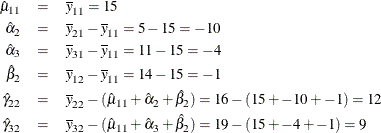
Figure 101.53: Reference Cell Model, (1,1) Reference Cell, Design Matrix
| Two-Way ANOVA Models |
| Reference Cell Model, (1,1) Reference Cell |
| Obs | _TYPE_ | _NAME_ | y | Intercept | a 2 | a 3 | b 2 | a 2 * b 2 |
a 3 * b 2 |
a | b |
|---|---|---|---|---|---|---|---|---|---|---|---|
| 1 | SCORE | ROW1 | 16 | 1 | 0 | 0 | 0 | 0 | 0 | 1 | 1 |
| 2 | SCORE | ROW2 | 14 | 1 | 0 | 0 | 0 | 0 | 0 | 1 | 1 |
| 3 | SCORE | ROW3 | 15 | 1 | 0 | 0 | 1 | 0 | 0 | 1 | 2 |
| 4 | SCORE | ROW4 | 13 | 1 | 0 | 0 | 1 | 0 | 0 | 1 | 2 |
| 5 | SCORE | ROW5 | 1 | 1 | 1 | 0 | 0 | 0 | 0 | 2 | 1 |
| 6 | SCORE | ROW6 | 9 | 1 | 1 | 0 | 0 | 0 | 0 | 2 | 1 |
| 7 | SCORE | ROW7 | 12 | 1 | 1 | 0 | 1 | 1 | 0 | 2 | 2 |
| 8 | SCORE | ROW8 | 20 | 1 | 1 | 0 | 1 | 1 | 0 | 2 | 2 |
| 9 | SCORE | ROW9 | 14 | 1 | 0 | 1 | 0 | 0 | 0 | 3 | 1 |
| 10 | SCORE | ROW10 | 8 | 1 | 0 | 1 | 0 | 0 | 0 | 3 | 1 |
| 11 | SCORE | ROW11 | 18 | 1 | 0 | 1 | 1 | 0 | 1 | 3 | 2 |
| 12 | SCORE | ROW12 | 20 | 1 | 0 | 1 | 1 | 0 | 1 | 3 | 2 |
The next model is a deviations-from-means model, but this time the reference cell is the first cell (1,1). This coding is also called effects coding. The following statements produce Figure 101.54 and Figure 101.55:
proc transreg data=x ss2 short;
   title2 'Deviations from Means, (1,1) Reference Cell';
   model identity(y) = class(a | b / deviations zero=first);
   output replace;
run;

proc print label;
run;
Figure 101.54: Deviations-from-Means Model, (1,1) Reference Cell
| Two-Way ANOVA Models |
| Deviations from Means, (1,1) Reference Cell |
| Dependent Variable Identity(y) |
| Class Level Information | ||
|---|---|---|
| Class | Levels | Values |
| a | 3 | 1 2 3 |
| b | 2 | 1 2 |
| Number of Observations Read | 12 |
|---|---|
| Number of Observations Used | 12 |
| The TRANSREG Procedure Hypothesis Tests for Identity(y) |
| Univariate ANOVA Table Based on the Usual Degrees of Freedom | |||||
|---|---|---|---|---|---|
| Source | DF | Sum of Squares | Mean Square | F Value | Pr > F |
| Model | 5 | 234.6667 | 46.93333 | 3.20 | 0.0946 |
| Error | 6 | 88.0000 | 14.66667 | ||
| Corrected Total | 11 | 322.6667 | |||
| Root MSE | 3.82971 | R-Square | 0.7273 |
|---|---|---|---|
| Dependent Mean | 13.33333 | Adj R-Sq | 0.5000 |
| Coeff Var | 28.72281 |
| Univariate Regression Table Based on the Usual Degrees of Freedom | |||||||
|---|---|---|---|---|---|---|---|
| Variable | DF | Coefficient | Type II Sum of Squares |
Mean Square | F Value | Pr > F | Label |
| Intercept | 1 | 13.3333333 | 2133.33 | 2133.33 | 145.45 | <.0001 | Intercept |
| Class.a2 | 1 | -2.8333333 | 48.17 | 48.17 | 3.28 | 0.1199 | a 2 |
| Class.a3 | 1 | 1.6666667 | 16.67 | 16.67 | 1.14 | 0.3274 | a 3 |
| Class.b2 | 1 | 3.0000000 | 108.00 | 108.00 | 7.36 | 0.0349 | b 2 |
| Class.a2b2 | 1 | 2.5000000 | 37.50 | 37.50 | 2.56 | 0.1609 | a 2 * b 2 |
| Class.a3b2 | 1 | 1.0000000 | 6.00 | 6.00 | 0.41 | 0.5461 | a 3 * b 2 |
Notice that all of the parameter estimates match the corresponding estimates from the less-than-full-rank coding.
Figure 101.55: Deviations-from-Means Model, (1,1) Reference Cell, Design Matrix
| Two-Way ANOVA Models |
| Deviations from Means, (1,1) Reference Cell |
| Obs | _TYPE_ | _NAME_ | y | Intercept | a 2 | a 3 | b 2 | a 2 * b 2 | a 3 * b 2 | a | b |
|---|---|---|---|---|---|---|---|---|---|---|---|
| 1 | SCORE | ROW1 | 16 | 1 | -1 | -1 | -1 | 1 | 1 | 1 | 1 |
| 2 | SCORE | ROW2 | 14 | 1 | -1 | -1 | -1 | 1 | 1 | 1 | 1 |
| 3 | SCORE | ROW3 | 15 | 1 | -1 | -1 | 1 | -1 | -1 | 1 | 2 |
| 4 | SCORE | ROW4 | 13 | 1 | -1 | -1 | 1 | -1 | -1 | 1 | 2 |
| 5 | SCORE | ROW5 | 1 | 1 | 1 | 0 | -1 | -1 | 0 | 2 | 1 |
| 6 | SCORE | ROW6 | 9 | 1 | 1 | 0 | -1 | -1 | 0 | 2 | 1 |
| 7 | SCORE | ROW7 | 12 | 1 | 1 | 0 | 1 | 1 | 0 | 2 | 2 |
| 8 | SCORE | ROW8 | 20 | 1 | 1 | 0 | 1 | 1 | 0 | 2 | 2 |
| 9 | SCORE | ROW9 | 14 | 1 | 0 | 1 | -1 | 0 | -1 | 3 | 1 |
| 10 | SCORE | ROW10 | 8 | 1 | 0 | 1 | -1 | 0 | -1 | 3 | 1 |
| 11 | SCORE | ROW11 | 18 | 1 | 0 | 1 | 1 | 0 | 1 | 3 | 2 |
| 12 | SCORE | ROW12 | 20 | 1 | 0 | 1 | 1 | 0 | 1 | 3 | 2 |
The following statements fit a model with an orthogonal-contrast coding and produce Figure 101.56 and Figure 101.57:
proc transreg data=x ss2 short;
   title2 'Orthogonal Contrast Coding';
   model identity(y) = class(a | b / orthogonal);
   output replace;
run;

proc print label;
run;
Figure 101.56: Orthogonal-Contrast Coding
| Two-Way ANOVA Models |
| Orthogonal Contrast Coding |
| Dependent Variable Identity(y) |
| Class Level Information | ||
|---|---|---|
| Class | Levels | Values |
| a | 3 | 1 2 3 |
| b | 2 | 1 2 |
| Number of Observations Read | 12 |
|---|---|
| Number of Observations Used | 12 |
| The TRANSREG Procedure Hypothesis Tests for Identity(y) |
| Univariate ANOVA Table Based on the Usual Degrees of Freedom | |||||
|---|---|---|---|---|---|
| Source | DF | Sum of Squares | Mean Square | F Value | Pr > F |
| Model | 5 | 234.6667 | 46.93333 | 3.20 | 0.0946 |
| Error | 6 | 88.0000 | 14.66667 | ||
| Corrected Total | 11 | 322.6667 | |||
| Root MSE | 3.82971 | R-Square | 0.7273 |
|---|---|---|---|
| Dependent Mean | 13.33333 | Adj R-Sq | 0.5000 |
| Coeff Var | 28.72281 |
| Univariate Regression Table Based on the Usual Degrees of Freedom | |||||||
|---|---|---|---|---|---|---|---|
| Variable | DF | Coefficient | Type II Sum of Squares |
Mean Square | F Value | Pr > F | Label |
| Intercept | 1 | 13.3333333 | 2133.33 | 2133.33 | 145.45 | <.0001 | Intercept |
| Class.a1 | 1 | -0.2500000 | 0.50 | 0.50 | 0.03 | 0.8596 | a 1 |
| Class.a2 | 1 | -1.4166667 | 48.17 | 48.17 | 3.28 | 0.1199 | a 2 |
| Class.b1 | 1 | -3.0000000 | 108.00 | 108.00 | 7.36 | 0.0349 | b 1 |
| Class.a1b1 | 1 | 2.2500000 | 40.50 | 40.50 | 2.76 | 0.1476 | a 1 * b 1 |
| Class.a2b1 | 1 | -1.2500000 | 37.50 | 37.50 | 2.56 | 0.1609 | a 2 * b 1 |
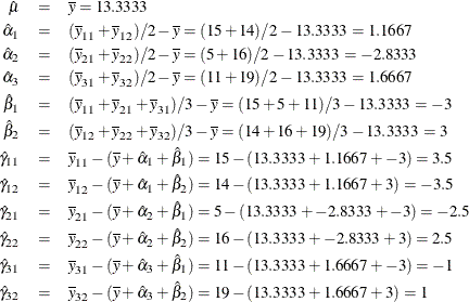
The parameter estimates are

Figure 101.57: Orthogonal-Contrast Coding, Design Matrix
| Two-Way ANOVA Models |
| Orthogonal Contrast Coding |
| Obs | _TYPE_ | _NAME_ | y | Intercept | a 1 | a 2 | b 1 | a 1 * b 1 | a 2 * b 1 | a | b |
|---|---|---|---|---|---|---|---|---|---|---|---|
| 1 | SCORE | ROW1 | 16 | 1 | 1 | -1 | 1 | 1 | -1 | 1 | 1 |
| 2 | SCORE | ROW2 | 14 | 1 | 1 | -1 | 1 | 1 | -1 | 1 | 1 |
| 3 | SCORE | ROW3 | 15 | 1 | 1 | -1 | -1 | -1 | 1 | 1 | 2 |
| 4 | SCORE | ROW4 | 13 | 1 | 1 | -1 | -1 | -1 | 1 | 1 | 2 |
| 5 | SCORE | ROW5 | 1 | 1 | 0 | 2 | 1 | 0 | 2 | 2 | 1 |
| 6 | SCORE | ROW6 | 9 | 1 | 0 | 2 | 1 | 0 | 2 | 2 | 1 |
| 7 | SCORE | ROW7 | 12 | 1 | 0 | 2 | -1 | 0 | -2 | 2 | 2 |
| 8 | SCORE | ROW8 | 20 | 1 | 0 | 2 | -1 | 0 | -2 | 2 | 2 |
| 9 | SCORE | ROW9 | 14 | 1 | -1 | -1 | 1 | -1 | -1 | 3 | 1 |
| 10 | SCORE | ROW10 | 8 | 1 | -1 | -1 | 1 | -1 | -1 | 3 | 1 |
| 11 | SCORE | ROW11 | 18 | 1 | -1 | -1 | -1 | 1 | 1 | 3 | 2 |
| 12 | SCORE | ROW12 | 20 | 1 | -1 | -1 | -1 | 1 | 1 | 3 | 2 |
The following statements fit a model with a standardized-orthogonal coding and produce Figure 101.58 and Figure 101.59:
proc transreg data=x ss2 short;
   title2 'Standardized-Orthogonal Coding';
   model identity(y) = class(a | b / standorth);
   output replace;
run;

proc print label;
run;
Figure 101.58: Standardized-Orthogonal Coding
| Two-Way ANOVA Models |
| Standardized-Orthogonal Coding |
| Dependent Variable Identity(y) |
| Class Level Information | ||
|---|---|---|
| Class | Levels | Values |
| a | 3 | 1 2 3 |
| b | 2 | 1 2 |
| Number of Observations Read | 12 |
|---|---|
| Number of Observations Used | 12 |
| The TRANSREG Procedure Hypothesis Tests for Identity(y) |
| Univariate ANOVA Table Based on the Usual Degrees of Freedom | |||||
|---|---|---|---|---|---|
| Source | DF | Sum of Squares | Mean Square | F Value | Pr > F |
| Model | 5 | 234.6667 | 46.93333 | 3.20 | 0.0946 |
| Error | 6 | 88.0000 | 14.66667 | ||
| Corrected Total | 11 | 322.6667 | |||
| Root MSE | 3.82971 | R-Square | 0.7273 |
|---|---|---|---|
| Dependent Mean | 13.33333 | Adj R-Sq | 0.5000 |
| Coeff Var | 28.72281 |
| Univariate Regression Table Based on the Usual Degrees of Freedom | |||||||
|---|---|---|---|---|---|---|---|
| Variable | DF | Coefficient | Type II Sum of Squares |
Mean Square | F Value | Pr > F | Label |
| Intercept | 1 | 13.3333333 | 2133.33 | 2133.33 | 145.45 | <.0001 | Intercept |
| Class.a1 | 1 | -0.2041241 | 0.50 | 0.50 | 0.03 | 0.8596 | a 1 |
| Class.a2 | 1 | -2.0034692 | 48.17 | 48.17 | 3.28 | 0.1199 | a 2 |
| Class.b1 | 1 | -3.0000000 | 108.00 | 108.00 | 7.36 | 0.0349 | b 1 |
| Class.a1b1 | 1 | 1.8371173 | 40.50 | 40.50 | 2.76 | 0.1476 | a 1 * b 1 |
| Class.a2b1 | 1 | -1.7677670 | 37.50 | 37.50 | 2.56 | 0.1609 | a 2 * b 1 |
The parameter estimates are
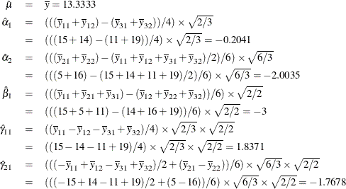
The numerators in the square roots are sums of squares of the coded values for the unstandardized-orthogonal codings, and
the denominators are the numbers of levels. These terms convert the estimates from the orthogonal contrast coding to the standardized-orthogonal
coding. The term ![]() , which is 1 and could be dropped, is included in the preceding formulas to show the general pattern. Notice the regression
tables for the orthogonal-contrast coding and the standardized-orthogonal coding. Some of the coefficients are different,
but the rest of the table is the same since the coded variables for the two models differ only by a constant.
, which is 1 and could be dropped, is included in the preceding formulas to show the general pattern. Notice the regression
tables for the orthogonal-contrast coding and the standardized-orthogonal coding. Some of the coefficients are different,
but the rest of the table is the same since the coded variables for the two models differ only by a constant.
Figure 101.59: Standardized-Orthogonal Coding, Design Matrix
| Two-Way ANOVA Models |
| Standardized-Orthogonal Coding |
| Obs | _TYPE_ | _NAME_ | y | Intercept | a 1 | a 2 | b 1 | a 1 * b 1 | a 2 * b 1 | a | b |
|---|---|---|---|---|---|---|---|---|---|---|---|
| 1 | SCORE | ROW1 | 16 | 1 | 1.22474 | -0.70711 | 1 | 1.22474 | -0.70711 | 1 | 1 |
| 2 | SCORE | ROW2 | 14 | 1 | 1.22474 | -0.70711 | 1 | 1.22474 | -0.70711 | 1 | 1 |
| 3 | SCORE | ROW3 | 15 | 1 | 1.22474 | -0.70711 | -1 | -1.22474 | 0.70711 | 1 | 2 |
| 4 | SCORE | ROW4 | 13 | 1 | 1.22474 | -0.70711 | -1 | -1.22474 | 0.70711 | 1 | 2 |
| 5 | SCORE | ROW5 | 1 | 1 | 0.00000 | 1.41421 | 1 | 0.00000 | 1.41421 | 2 | 1 |
| 6 | SCORE | ROW6 | 9 | 1 | 0.00000 | 1.41421 | 1 | 0.00000 | 1.41421 | 2 | 1 |
| 7 | SCORE | ROW7 | 12 | 1 | 0.00000 | 1.41421 | -1 | 0.00000 | -1.41421 | 2 | 2 |
| 8 | SCORE | ROW8 | 20 | 1 | 0.00000 | 1.41421 | -1 | 0.00000 | -1.41421 | 2 | 2 |
| 9 | SCORE | ROW9 | 14 | 1 | -1.22474 | -0.70711 | 1 | -1.22474 | -0.70711 | 3 | 1 |
| 10 | SCORE | ROW10 | 8 | 1 | -1.22474 | -0.70711 | 1 | -1.22474 | -0.70711 | 3 | 1 |
| 11 | SCORE | ROW11 | 18 | 1 | -1.22474 | -0.70711 | -1 | 1.22474 | 0.70711 | 3 | 2 |
| 12 | SCORE | ROW12 | 20 | 1 | -1.22474 | -0.70711 | -1 | 1.22474 | 0.70711 | 3 | 2 |