The VARMAX Procedure
- Overview
-
Getting Started

-
Syntax
-
DetailsMissing ValuesVARMAX ModelDynamic Simultaneous Equations ModelingImpulse Response FunctionForecastingTentative Order SelectionVAR and VARX ModelingSeasonal Dummies and Time TrendsBayesian VAR and VARX ModelingVARMA and VARMAX ModelingModel Diagnostic ChecksCointegrationVector Error Correction ModelingI(2) ModelVector Error Correction Model in ARMA FormMultivariate GARCH ModelingOutput Data SetsOUT= Data SetOUTEST= Data SetOUTHT= Data SetOUTSTAT= Data SetPrinted OutputODS Table NamesODS GraphicsComputational Issues
-
Examples
- References
Model Diagnostic Checks
Multivariate Model Diagnostic Checks
Log Likelihood
The log-likelihood function for the fitted model is reported in the LogLikelihood ODS table. The log-likelihood functions for different models are defined as follows:
-
For VARMAX models that are estimated through the (conditional) maximum likelihood method, see the section VARMA and VARMAX Modeling.
-
For Bayesian VAR and VARX models, see the section Bayesian VAR and VARX Modeling.
-
For (Bayesian) vector error correction models, see the section Vector Error Correction Modeling.
-
For multivariate GARCH models, see the section Multivariate GARCH Modeling.
-
For VAR and VARX models that are estimated through the least squares (LS) method, the log likelihood is defined as
![\[ \ell = -\frac{1}{2}(T \log |\tilde{\Sigma }| + k T) \]](images/etsug_varmax0693.png)
where
 is the maximum likelihood estimate of the innovation covariance matrix, k is the number of dependent variables, and T is the number of observations used in the estimation.
Information Criteria
The information criteria include Akaike’s information criterion (AIC), the corrected Akaike’s information criterion (AICC), the final prediction error criterion (FPE), the Hannan-Quinn criterion (HQC), and the Schwarz Bayesian criterion (SBC, also referred to as BIC). These criteria are defined as
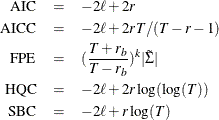
where  is the log likelihood, r is the total number of parameters in the model, k is the number of dependent variables, T is the number of observations that are used to estimate the model,
  is the number of parameters in each mean equation, and is the maximum likelihood estimate of
  . As suggested by Burnham and Anderson (2004) for least squares estimation, the total number of parameters, r, must include the parameters in the innovation covariance matrix. When comparing models, choose the model that has the smallest
criterion values.
. As suggested by Burnham and Anderson (2004) for least squares estimation, the total number of parameters, r, must include the parameters in the innovation covariance matrix. When comparing models, choose the model that has the smallest
criterion values.
See Figure 42.4 earlier in this chapter for an example of the output.
Portmanteau Statistic
The Portmanteau statistic,  , is used to test whether correlation remains on the model residuals. The null hypothesis is that the residuals are uncorrelated.
Let
, is used to test whether correlation remains on the model residuals. The null hypothesis is that the residuals are uncorrelated.
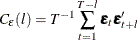
Let  be the residual cross-covariance matrices,
  be the residual cross-correlation matrices as
and

where 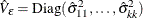 and
and  are the diagonal elements of
  . The multivariate portmanteau test defined in Hosking (1980) is
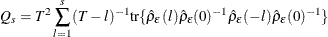
The statistic has approximately the chi-square distribution with  degrees of freedom. An example of the output is displayed in Figure 42.7.
Univariate Model Diagnostic Checks
There are various ways to perform diagnostic checks for a univariate model. For details, see the section Testing for Nonlinear Dependence: Heteroscedasticity Tests in Chapter 9: The AUTOREG Procedure. An example of the output is displayed in Figure 42.8 and Figure 42.9.
-
Durbin-Watson (DW) statistics: The DW test statistics test for the first order autocorrelation in the residuals.
-
Jarque-Bera normality test: This test is helpful in determining whether the model residuals represent a white noise process. This tests the null hypothesis that the residuals have normality.
-
F tests for autoregressive conditional heteroscedastic (ARCH) disturbances: F test statistics test for the heteroscedastic disturbances in the residuals. This tests the null hypothesis that the residuals have equal covariances
-
F tests for AR disturbance: These test statistics are computed from the residuals of the univariate AR(1), AR(1,2), AR(1,2,3) and AR(1,2,3,4) models to test the null hypothesis that the residuals are uncorrelated.