The VARMAX Procedure
- Overview
-
Getting Started

-
Syntax
-
DetailsMissing ValuesVARMAX ModelDynamic Simultaneous Equations ModelingImpulse Response FunctionForecastingTentative Order SelectionVAR and VARX ModelingSeasonal Dummies and Time TrendsBayesian VAR and VARX ModelingVARMA and VARMAX ModelingModel Diagnostic ChecksCointegrationVector Error Correction ModelingI(2) ModelVector Error Correction Model in ARMA FormMultivariate GARCH ModelingOutput Data SetsOUT= Data SetOUTEST= Data SetOUTHT= Data SetOUTSTAT= Data SetPrinted OutputODS Table NamesODS GraphicsComputational Issues
-
Examples
- References
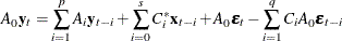
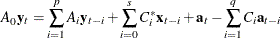
Dynamic Simultaneous Equations Modeling
In the econometrics literature, the VARMAX(p,q,s) model is sometimes written in a form that is slightly different than the one shown in the previous section. This alternative form is referred to as a dynamic simultaneous equations model or a dynamic structural equations model.
Because  is assumed to be positive-definite, there exists a lower triangular matrix
  that has ones on the diagonals such that
  , where
  is a diagonal matrix that has positive diagonal elements.
where  ,
,  , and
, and  .
.
As an alternative form,
where , , , and  . The covariance matrix of
  is the diagonal matrix . The PRINT=(DYNAMIC) option returns the parameter estimates that result from estimating the model in this form.
A dynamic simultaneous equations model involves a leading (lower triangular) coefficient matrix for  at lag 0 or a leading coefficient matrix for
  at lag 0. Such a representation of the VARMAX(p,q,s) model can be more useful in certain circumstances than the standard representation. From the linear combination of the dependent
variables obtained by
at lag 0. Such a representation of the VARMAX(p,q,s) model can be more useful in certain circumstances than the standard representation. From the linear combination of the dependent
variables obtained by  , you can easily see the relationship between the dependent variables in the current time.
The following statements provide the dynamic simultaneous equations of the VAR(1) model.
proc iml;
   sig = {1.0  0.5, 0.5 1.25};
   phi = {1.2 -0.5, 0.6 0.3};
   /* simulate the vector time series */
   call varmasim(y,phi) sigma = sig n = 100 seed = 34657;
   cn = {'y1' 'y2'};
   create simul1 from y[colname=cn];
   append from y;
quit;

data simul1;
   set simul1;
   date = intnx( 'year', '01jan1900'd, _n_-1 );
   format date year4.;
run;
proc varmax data=simul1;
   model y1 y2 / p=1 noint print=(dynamic);
run;
This is the same data set and model used in the section Getting Started: VARMAX Procedure. You can compare the results of the VARMA model form and the dynamic simultaneous equations model form.
Figure 42.40: Dynamic Simultaneous Equations (DYNAMIC Option)
| Covariances of Innovations | ||
|---|---|---|
| Variable | y1 | y2 |
| y1 | 1.28875 | 0.00000 |
| y2 | 0.00000 | 1.29578 |
| AR | |||
|---|---|---|---|
| Lag | Variable | y1 | y2 |
| 0 | y1 | 1.00000 | 0.00000 |
| y2 | -0.30845 | 1.00000 | |
| 1 | y1 | 1.15977 | -0.51058 |
| y2 | 0.18861 | 0.54247 | |
| Dynamic Model Parameter Estimates | ||||||
|---|---|---|---|---|---|---|
| Equation | Parameter | Estimate | Standard Error |
t Value | Pr > |t| | Variable |
| y1 | AR1_1_1 | 1.15977 | 0.05508 | 21.06 | 0.0001 | y1(t-1) |
| AR1_1_2 | -0.51058 | 0.07140 | -7.15 | 0.0001 | y2(t-1) | |
| y2 | AR0_2_1 | 0.30845 | y1(t) | |||
| AR1_2_1 | 0.18861 | 0.05779 | 3.26 | 0.0015 | y1(t-1) | |
| AR1_2_2 | 0.54247 | 0.07491 | 7.24 | 0.0001 | y2(t-1) | |
In Figure 42.4 in the section Getting Started: VARMAX Procedure, the covariance of estimated from the VARMAX model form is
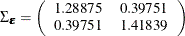
Figure 42.40 shows the results from estimating the model as a dynamic simultaneous equations model. By the decomposition of  , you get a diagonal matrix (
 ) and a lower triangular matrix () such as
  where
where

The lower triangular matrix () is shown in the left side of the simultaneous equations model. The parameter estimates in equations system are shown in
the right side of the two-equations system.
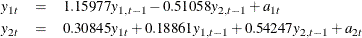
The simultaneous equations model is written as

The resulting two-equation system can be written as