The VARMAX Procedure
- Overview
-
Getting Started

-
Syntax
-
DetailsMissing ValuesVARMAX ModelDynamic Simultaneous Equations ModelingImpulse Response FunctionForecastingTentative Order SelectionVAR and VARX ModelingSeasonal Dummies and Time TrendsBayesian VAR and VARX ModelingVARMA and VARMAX ModelingModel Diagnostic ChecksCointegrationVector Error Correction ModelingI(2) ModelVector Error Correction Model in ARMA FormMultivariate GARCH ModelingOutput Data SetsOUT= Data SetOUTEST= Data SetOUTHT= Data SetOUTSTAT= Data SetPrinted OutputODS Table NamesODS GraphicsComputational Issues
-
Examples
- References
Vector Autoregressive Model
Let 
 denote a k-dimensional time series vector of random variables of interest. The pth-order VAR process is written as

where  is a vector white noise process such that
  ,
,  , and
, and  for
for  ;
;  is a constant vector; and
  is a
is a  matrix.
Analyzing and modeling the series jointly enables you to understand the dynamic relationships over time among the series and to improve the accuracy of forecasts for individual series by using the additional information available from the related series and their forecasts.
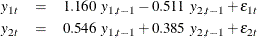
Consider the first-order stationary bivariate vector autoregressive model:

The following IML procedure statements simulate a bivariate vector time series from this model to provide test data for the VARMAX procedure:
proc iml;
   sig = {1.0  0.5, 0.5 1.25};
   phi = {1.2 -0.5, 0.6 0.3};
   /* simulate the vector time series */
   call varmasim(y,phi) sigma = sig n = 100 seed = 34657;
   cn = {'y1' 'y2'};
   create simul1 from y[colname=cn];
   append from y;
quit;
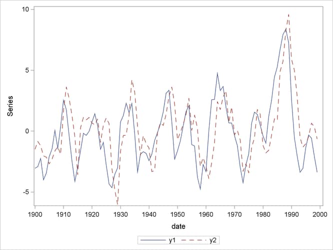
The following statements plot the simulated vector time series  , which is shown in Figure 42.1:
data simul1;
   set simul1;
   date = intnx( 'year', '01jan1900'd, _n_-1 );
   format date year4.;
run;

proc sgplot data=simul1;
   series x=date y=y1 / lineattrs=(pattern=solid);
   series x=date y=y2 / lineattrs=(pattern=dash);
   yaxis label="Series";
run;
Figure 42.1: Plot of the Generated Data Process
The following statements fit a VAR(1) model to the simulated data:
/*--- Vector Autoregressive Model ---*/

proc varmax data=simul1;
   id date interval=year;
   model y1 y2 / p=1 noint lagmax=3
                 print=(estimates diagnose);
   output out=for lead=5;
run;
First, you specify the input data set in the PROC VARMAX statement. Then, you use the MODEL statement to designate the dependent
variables,  and
and  . To estimate a zero-mean VAR model, you specify the order of the autoregressive model in the P= option and the NOINT option.
The MODEL statement fits the model to the data and prints parameter estimates and their significance. The PRINT=ESTIMATES
option prints the matrix form of parameter estimates, and the PRINT=DIAGNOSE option prints various diagnostic tests. The LAGMAX=3
option prints the output for the residual diagnostic checks.
. To estimate a zero-mean VAR model, you specify the order of the autoregressive model in the P= option and the NOINT option.
The MODEL statement fits the model to the data and prints parameter estimates and their significance. The PRINT=ESTIMATES
option prints the matrix form of parameter estimates, and the PRINT=DIAGNOSE option prints various diagnostic tests. The LAGMAX=3
option prints the output for the residual diagnostic checks.
To output the forecasts to a data set, you specify the OUT= option in the OUTPUT statement. If you want to forecast five steps ahead, you use the LEAD=5 option. The ID statement specifies the yearly interval between observations and provides the Time column in the forecast output.
The VARMAX procedure output is shown in Figure 42.2 through Figure 42.10. The VARMAX procedure first displays descriptive statistics, as shown in Figure 42.2. The Type column indicates that the variables are dependent variables. The N column indicates the number of nonmissing observations.
Figure 42.2: Descriptive Statistics
Figure 42.3 shows the model type and the estimation method that is used to fit the model to the simulated data. It also shows the AR coefficient matrix in terms of lag 1, the schematic representation, and the parameter estimates and their significance that can indicate how well the model fits the data.
The "AR" table shows the AR coefficient matrix. The "Schematic Representation" table schematically represents the parameter estimates and enables you to easily verify their significance in matrix form.
In the "Model Parameter Estimates" table, the first column shows the variable on the left side of the equation; the second
column is the parameter name AR , which indicates the (i, j) element of the lag l autoregressive coefficient; the next four columns provide the estimate, standard error, t value, and p-value for the parameter; and the last column is the regressor that corresponds to the displayed parameter.
Figure 42.3: Model Type and Parameter Estimates
| Type of Model | VAR(1) |
|---|---|
| Estimation Method | Least Squares Estimation |
| AR | |||
|---|---|---|---|
| Lag | Variable | y1 | y2 |
| 1 | y1 | 1.15977 | -0.51058 |
| y2 | 0.54634 | 0.38499 | |
| Schematic Representation |
|
|---|---|
| Variable/Lag | AR1 |
| y1 | +- |
| y2 | ++ |
| + is > 2*std error, - is < -2*std error, . is between, * is N/A | |
| Model Parameter Estimates | ||||||
|---|---|---|---|---|---|---|
| Equation | Parameter | Estimate | Standard Error |
t Value | Pr > |t| | Variable |
| y1 | AR1_1_1 | 1.15977 | 0.05508 | 21.06 | 0.0001 | y1(t-1) |
| AR1_1_2 | -0.51058 | 0.05898 | -8.66 | 0.0001 | y2(t-1) | |
| y2 | AR1_2_1 | 0.54634 | 0.05779 | 9.45 | 0.0001 | y1(t-1) |
| AR1_2_2 | 0.38499 | 0.06188 | 6.22 | 0.0001 | y2(t-1) | |
The fitted VAR(1) model with estimated standard errors in parentheses is given as
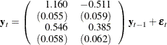
Clearly, all parameter estimates in the coefficient matrix  are significant.
The model can also be written as two univariate regression equations:
The table in Figure 42.4 shows the innovation covariance matrix estimates, the log likelihood, and the various information criteria results. The variable
names in the table for the innovation covariance matrix estimates  are printed for convenience:
  means the innovation for , and
  means the innovation for . The log likelihood for a VAR model that is estimated through least squares method is defined as
 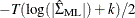 , where
 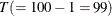 is the sample size except the presample being skipped because of the AR lag order,
  is the number of dependent variables, and
  is the maximum likelihood estimate (MLE) of innovation covariance matrix. The matrix is computed from the reported least squares estimate of the innovation covariance matrix, , by adjusting the degrees of freedom.
  , where
  is the number of parameters in each equation. You can use the information criteria to compare the fit of competing models
to a set of data. The model that has a smaller value of the information criterion is preferred when it is compared to other
models. For more information about how to calculate the information criteria, see the section Multivariate Model Diagnostic Checks.
is the number of parameters in each equation. You can use the information criteria to compare the fit of competing models
to a set of data. The model that has a smaller value of the information criterion is preferred when it is compared to other
models. For more information about how to calculate the information criteria, see the section Multivariate Model Diagnostic Checks.
Figure 42.4: Innovation Covariance Estimates, Log Likelihood, and Information Criteria
Figure 42.5 shows the cross covariances of the residuals. The values of the lag 0 are slightly different from Figure 42.4 because of the different degrees of freedom.
Figure 42.5: Multivariate Diagnostic Checks
Figure 42.6 and Figure 42.7 show tests for white noise residuals that are based on the cross correlations of the residuals. The output shows that you cannot reject the null hypothesis that the residuals are uncorrelated.
Figure 42.6: Multivariate Diagnostic Checks, Continued
| Cross Correlations of Residuals | |||
|---|---|---|---|
| Lag | Variable | y1 | y2 |
| 0 | y1 | 1.00000 | 0.29401 |
| y2 | 0.29401 | 1.00000 | |
| 1 | y1 | 0.02472 | 0.04284 |
| y2 | -0.03507 | -0.03884 | |
| 2 | y1 | 0.06442 | 0.08001 |
| y2 | 0.02628 | -0.01115 | |
| 3 | y1 | 0.01302 | 0.08858 |
| y2 | 0.00460 | 0.08213 | |
| Schematic Representation of Cross Correlations of Residuals |
||||
|---|---|---|---|---|
| Variable/Lag | 0 | 1 | 2 | 3 |
| y1 | ++ | .. | .. | .. |
| y2 | ++ | .. | .. | .. |
| + is > 2*std error, - is < -2*std error, . is between | ||||
Figure 42.7: Multivariate Diagnostic Checks, Continued
The VARMAX procedure provides diagnostic checks for the univariate form of the equations. The table in Figure 42.8 describes how well each univariate equation fits the data. From the two univariate regression equations shown in Figure 42.3, the values of  in the second column of Figure 42.8 are 0.84 and 0.79. The standard deviations in the third column are the square roots of the diagonal elements of the covariance
matrix from Figure 42.4. The F statistics in the fourth column test the null hypotheses
in the second column of Figure 42.8 are 0.84 and 0.79. The standard deviations in the third column are the square roots of the diagonal elements of the covariance
matrix from Figure 42.4. The F statistics in the fourth column test the null hypotheses  and
and  , where
  is the (i, j) element of the matrix . The last column shows the p-values of the F statistics. The results show that each univariate model is significant.
Figure 42.8: Univariate Diagnostic Checks
The check for white noise residuals in terms of the univariate equation is shown in Figure 42.9. This output contains information that indicates whether the residuals are correlated and heteroscedastic. In the first table, the second column contains the Durbin-Watson test statistics to test the null hypothesis that the residuals are uncorrelated. The third and fourth columns show the Jarque-Bera normality test statistics and their p-values to test the null hypothesis that the residuals have normality. The last two columns show F statistics and their p-values for ARCH(1) disturbances to test the null hypothesis that the residuals have equal covariances. The second table includes F statistics and their p-values for AR(1), AR(1,2), AR(1,2,3) and AR(1,2,3,4) models of residuals to test the null hypothesis that the residuals are uncorrelated.
Figure 42.9: Univariate Diagnostic Checks, Continued
| Univariate Model White Noise Diagnostics | |||||
|---|---|---|---|---|---|
| Variable | Durbin Watson |
Normality | ARCH | ||
| Chi-Square | Pr > ChiSq | F Value | Pr > F | ||
| y1 | 1.94534 | 3.56 | 0.1686 | 0.13 | 0.7199 |
| y2 | 2.06276 | 5.42 | 0.0667 | 2.10 | 0.1503 |
| Univariate Model AR Diagnostics | ||||||||
|---|---|---|---|---|---|---|---|---|
| Variable | AR1 | AR2 | AR3 | AR4 | ||||
| F Value | Pr > F | F Value | Pr > F | F Value | Pr > F | F Value | Pr > F | |
| y1 | 0.02 | 0.8980 | 0.14 | 0.8662 | 0.09 | 0.9629 | 0.82 | 0.5164 |
| y2 | 0.52 | 0.4709 | 0.41 | 0.6650 | 0.32 | 0.8136 | 0.32 | 0.8664 |
The table in Figure 42.10 shows forecasts, their prediction errors, and 95% confidence limits. For more information, see the section Forecasting.
Figure 42.10: Forecasts
| Forecasts | ||||||
|---|---|---|---|---|---|---|
| Variable | Obs | Time | Forecast | Standard Error |
95% Confidence Limits | |
| y1 | 101 | 2000 | -3.59212 | 1.13523 | -5.81713 | -1.36711 |
| 102 | 2001 | -3.09448 | 1.70915 | -6.44435 | 0.25539 | |
| 103 | 2002 | -2.17433 | 2.14472 | -6.37792 | 2.02925 | |
| 104 | 2003 | -1.11395 | 2.43166 | -5.87992 | 3.65203 | |
| 105 | 2004 | -0.14342 | 2.58740 | -5.21463 | 4.92779 | |
| y2 | 101 | 2000 | -2.09873 | 1.19096 | -4.43298 | 0.23551 |
| 102 | 2001 | -2.77050 | 1.47666 | -5.66469 | 0.12369 | |
| 103 | 2002 | -2.75724 | 1.74212 | -6.17173 | 0.65725 | |
| 104 | 2003 | -2.24943 | 2.01925 | -6.20709 | 1.70823 | |
| 105 | 2004 | -1.47460 | 2.25169 | -5.88782 | 2.93863 | |