The VARMAX Procedure
- Overview
-
Getting Started

-
Syntax
-
DetailsMissing ValuesVARMAX ModelDynamic Simultaneous Equations ModelingImpulse Response FunctionForecastingTentative Order SelectionVAR and VARX ModelingSeasonal Dummies and Time TrendsBayesian VAR and VARX ModelingVARMA and VARMAX ModelingModel Diagnostic ChecksCointegrationVector Error Correction ModelingI(2) ModelVector Error Correction Model in ARMA FormMultivariate GARCH ModelingOutput Data SetsOUT= Data SetOUTEST= Data SetOUTHT= Data SetOUTSTAT= Data SetPrinted OutputODS Table NamesODS GraphicsComputational Issues
-
Examples
- References
VARMA and VARMAX Modeling
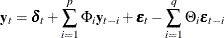
A zero-mean VARMA( ) process is written as
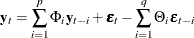
or
where  and
and  .
.
Stationarity and Invertibility
For stationarity and invertibility of the VARMA process, the roots of  and
and  are outside the unit circle.
Parameter Estimation
Under the assumption of normality of the  with zero-mean vector and nonsingular covariance matrix
  , the conditional (approximate) log-likelihood function of a zero-mean VARMA(p,q) model is considered.
Define  and
and  with
with  and
and  ; define
  and
and  . Then
![\[ \mb{y} -\sum _{i=1}^ p (I_ T \otimes \Phi _ i)B^ i \mb{y} =\mb{e} - \sum _{i=1}^ q (I_ T \otimes \Theta _ i)B^ i \mb{e} \]](images/etsug_varmax0624.png)
where ![$B^ i \mb{y} = \mr{vec} [(B^ i Y)’]$](images/etsug_varmax0625.png) and
and ![$B^ i \mb{e} = \mr{vec} [(B^ i E)’]$](images/etsug_varmax0626.png) .
.
Then, the conditional (approximate) log-likelihood function can be written as (Reinsel 1997)
where 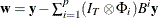 and
and  is such that
 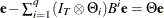 . You can specify METHOD=CML in the MODEL statement to apply conditional maximum likelihood estimation.
For the exact log-likelihood function of a VARMA model, the VARMA model is transformed into the equivalent state space form and then the Kalman filtering method is applied.
The state space form of the zero-mean VARMA(p,q) model consists of a state equation
![\[ \mb{z} _{t} =F\mb{z} _{t-1} + G\bepsilon _{t} \]](images/etsug_varmax0631.png)
and an observation equation
![\[ \mb{y} _ t = H\mb{z} _{t} \]](images/etsug_varmax0632.png)
where
![\[ \mb{z} _{t}=(\mb{y} _{t}’,\mb{y}_{t-1}’,\ldots ,\mb{y} _{t-(v-1)}’, \bepsilon _{t}’, \bepsilon _{t-1},\ldots ,\bepsilon _{t-(q-1)}’)’ \]](images/etsug_varmax0633.png)
![\[ F = \left[\begin{matrix} \Phi _{1} & \cdots & \Phi _{v-1} & \Phi _{v} & -\Theta _{1} & \cdots & -\Theta _{q-1} & -\Theta _{q} \\ I_ k & \cdots & 0 & 0 & 0 & \cdots & 0 & 0 \\ \vdots & \ddots & 0 & \vdots & \vdots & \ddots & \vdots & \vdots \\ 0 & \cdots & I_ k & 0 & 0 & \cdots & 0 & 0 \\ 0 & \cdots & 0 & 0 & 0 & \cdots & 0 & 0 \\ 0 & \cdots & 0 & 0 & I_ k & \cdots & 0 & 0 \\ \vdots & \ddots & 0 & \vdots & \vdots & \ddots & \vdots & \vdots \\ 0 & \cdots & 0 & 0 & 0 & \cdots & I_ k & 0 \\ \end{matrix} \right], ~ ~ G = \left[\begin{matrix} I_ k \\ 0_{k(v-1) \times k} \\ I_ k \\ 0_{k(q-1) \times k} \\ \end{matrix}\right] \]](images/etsug_varmax0634.png)
and
![\[ H = [I_ k, 0_{k(v+q-1) \times k}] \]](images/etsug_varmax0635.png)
where  and
and  for
for  .
.
The Kalman filtering approach is used to evaluate the likelihood function. The updating equation is
![\[ \hat{\mb{z}}_{t|t} = {\hat{\mb{z}}}_{t|t-1} + K_ t\bepsilon _{t|t-1} \]](images/etsug_varmax0639.png)
where
![\[ K_ t = P_{t|t-1}H’[H P_{t|t-1} H’]^{-1} \]](images/etsug_varmax0640.png)
The prediction equation is
![\[ \hat{\mb{z} }_{t|t-1} = F \hat{\mb{z} }_{t-1|t-1}, ~ ~ P_{t|t-1} = F P_{t-1|t-1} F’ + G \Sigma G’ \]](images/etsug_varmax0641.png)
where ![$P_{t|t} = [I-K_ tH]P_{t|t-1}$](images/etsug_varmax0642.png) for
for  .
.
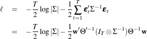
The log-likelihood function can be expressed as
![\[ \ell = -\frac{1}{2} \sum _{t=1}^ T [ \log |\Sigma _{t|t-1}| + (\mb{y} _{t}-\hat{\mb{y} }_{t|t-1})’\Sigma _{t|t-1}^{-1} (\mb{y} _{t}-\hat{\mb{y} }_{t|t-1}) ] \]](images/etsug_varmax0644.png)
where  and
and  are determined recursively from the Kalman filtering method. To construct the likelihood function from Kalman filtering,
you obtain
are determined recursively from the Kalman filtering method. To construct the likelihood function from Kalman filtering,
you obtain  ,
,  , and
, and 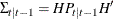 .
.
When you specify METHOD=ML in the MODEL statement, the exact log likelihood is evaluated and used in the maximum likelihood estimation.
Define the vector  as
as
![\[ \bbeta = ( \phi _1’, \ldots , \phi _ p’, \theta _1’, \ldots , \theta _ q’, \mr{vech} (\Sigma ) )’ \]](images/etsug_varmax0650.png)
where  and
and  . All elements of are estimated through the preceding (conditional) maximum likelihood method. The estimates of
  , and
, and  , are output in the ParameterEstimates ODS table. The estimates of the covariance matrix () are output in the CovarianceParameterEstimates ODS table. If you specify the OUTEST=, OUTCOV, PRINT=(COVB), or PRINT=(CORRB)
option, you can see all elements of , including the covariance matrix , in the parameter estimates, covariance of parameter estimates, or correlation of parameter estimates. You can also apply
the BOUND, INITIAL, RESTRICT, and TEST statements to any elements of , including the covariance matrix . For more information, see the syntax of the corresponding statement.
, are output in the ParameterEstimates ODS table. The estimates of the covariance matrix () are output in the CovarianceParameterEstimates ODS table. If you specify the OUTEST=, OUTCOV, PRINT=(COVB), or PRINT=(CORRB)
option, you can see all elements of , including the covariance matrix , in the parameter estimates, covariance of parameter estimates, or correlation of parameter estimates. You can also apply
the BOUND, INITIAL, RESTRICT, and TEST statements to any elements of , including the covariance matrix . For more information, see the syntax of the corresponding statement.
The (conditional) log-likelihood equations are solved by iterative numerical methods such as quasi-Newton optimization. The starting values for the AR and MA parameters are obtained from the least squares estimates. Although the small-sample properties of CML estimates might not be as good as the ML estimates, the CML method is much faster than the ML method. Depending on the sample size and number of parameters to be estimated, the CML method can be hundreds or even thousands of times faster than the ML method. In the following example code, the CML method is about 100 times faster than the ML method, with very similar estimation and forecast results:
proc iml;
   phi = (0.9 * I(4)) // (-0.7* I(4));
   theta = 0.8 * I(4);
   sig = I(4);

   /* to simulate the vector time series */
   call varmasim(y,phi,theta) sigma=sig n=400 seed=2;

   cn = {'y1' 'y2' 'y3' 'y4'};
   create simul6 from y[colname=cn];
   append from y;
   close;
quit;

proc varmax data=simul6;
   model y1 y2 y3 y4 / noint p=2 q=1 method=cml;
   nloptions pall maxit=5000 tech=qn;
   output out=ocml back=12 lead=24;
run;

proc varmax data=simul6;
   model y1 y2 y3 y4 / noint p=2 q=1 method=ml;
   nloptions pall maxit=5000 tech=qn;
   output out=oml back=12 lead=24;
run;
Asymptotic Distribution of the Parameter Estimates
Under the assumptions of stationarity and invertibility for the VARMA model and the assumption that is a white noise process,  is a consistent estimator for
  and
and  converges in distribution to the multivariate normal
  as
as  , where V is the asymptotic information matrix of .
Asymptotic Distributions of Impulse Response Functions
Defining the vector
![\[ \bbeta = ( \phi _1’, \ldots , \phi _ p’, \theta _1’, \ldots , \theta _ q’ )’ \]](images/etsug_varmax0659.png)
the asymptotic distribution of the impulse response function for a VARMA() model is
![\[ \sqrt {T} \mr{vec} (\hat\Psi _ j - \Psi _ j ) \stackrel{d}{\rightarrow } N(0, G_ j\Sigma _{\bbeta } G_ j’) ~ ~ j=1,2,\ldots \]](images/etsug_varmax0557.png)
where  is the covariance matrix of the parameter estimates and
![\[ G_ j= \frac{\partial \mr{vec} (\Psi _ j)}{\partial {\bbeta }'} = \sum _{i=0}^{j-1} \mb{H} ’(\mb{A} ’)^{j-1-i} \otimes \mb{J} \mb{A} ^ i\mb{J} ’ \]](images/etsug_varmax0661.png)
where ![$\mb{H} = [ I_ k, 0,\ldots , 0, I_ k, 0,\ldots , 0]’$](images/etsug_varmax0662.png) is a
is a  matrix with the second
  following after p block matrices;
 ![$\mb{J} = [ I_ k, 0,\ldots , 0 ]$](images/etsug_varmax0560.png) is a
is a  matrix;
  is a
is a 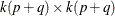 matrix,
![\begin{eqnarray*} \mb{A} = \left[\begin{matrix} A_{11} & A_{12} \\ A_{21} & A_{22} \\ \end{matrix}\right] \end{eqnarray*}](images/etsug_varmax0667.png)
where
![\begin{eqnarray*} A_{11} = \left[ \begin{matrix} \Phi _1 & \Phi _2 & \cdots & \Phi _{p-1} & \Phi _{p} \\ I_ k & 0 & \cdots & 0 & 0 \\ 0 & I_ k & \cdots & 0 & 0 \\ \vdots & \vdots & \ddots & \vdots & \vdots \\ 0 & 0 & \cdots & I_ k & 0 \\ \end{matrix} \right] ~ ~ A_{12} = \left[ \begin{matrix} -\Theta _1 & \cdots & -\Theta _{q-1} & -\Theta _{q} \\ 0 & \cdots & 0 & 0 \\ 0 & \cdots & 0 & 0 \\ \vdots & \ddots & \vdots & \vdots \\ 0 & \cdots & 0 & 0 \\ \end{matrix} \right] \end{eqnarray*}](images/etsug_varmax0668.png)
 is a
is a  zero matrix, and
![\begin{eqnarray*} A_{22} = \left[ \begin{matrix} 0 & 0 & \cdots & 0 & 0 \\ I_ k & 0 & \cdots & 0 & 0 \\ 0 & I_ k & \cdots & 0 & 0 \\ \vdots & \vdots & \ddots & \vdots & \vdots \\ 0 & 0 & \cdots & I_ k & 0 \\ \end{matrix} \right] \end{eqnarray*}](images/etsug_varmax0671.png)
An Example of a VARMA(1,1) Model
Consider a VARMA(1,1) model with mean zero,

where  is the white noise process with a mean zero vector and the positive-definite covariance matrix .
The following IML procedure statements simulate a bivariate vector time series from this model to provide test data for the VARMAX procedure:
proc iml;
   sig = {1.0  0.5, 0.5 1.25};
   phi = {1.2 -0.5, 0.6 0.3};
   theta = {0.5 -0.2, 0.1 0.3};
   /* to simulate the vector time series */
   call varmasim(y,phi,theta) sigma=sig n=100 seed=34657;
   cn = {'y1' 'y2'};
   create simul3 from y[colname=cn];
   append from y;
run;
The following statements fit a VARMA(1,1) model to the simulated data. You specify the order of the autoregressive model by using the P= option and specify the order of moving-average model by using the Q= option. You specify the quasi-Newton optimization in the NLOPTIONS statement as an optimization method.
proc varmax data=simul3;
   nloptions tech=qn;
   model y1 y2 / p=1 q=1 noint print=(estimates);
run;
Figure 42.62 shows the initial values of parameters. The initial values were estimated by using the least squares method.
Figure 42.62: Start Parameter Estimates for the VARMA(1, 1) Model
| Optimization Start | |||
|---|---|---|---|
| Parameter Estimates | |||
| N | Parameter | Estimate | Gradient Objective Function |
| 1 | AR1_1_1 | 0.964299 | -2.357098 |
| 2 | AR1_2_1 | 0.481620 | -3.773499 |
| 3 | AR1_1_2 | -0.363819 | 1.865051 |
| 4 | AR1_2_2 | 0.457378 | -10.778568 |
| 5 | MA1_1_1 | 0.244355 | -2.552198 |
| 6 | MA1_2_1 | -0.034093 | 2.716227 |
| 7 | MA1_1_2 | -0.006261 | -0.147004 |
| 8 | MA1_2_2 | 0.444636 | 0.141839 |
| 9 | COV1_1 | 1.353584 | 2.765550 |
| 10 | COV1_2 | 0.415649 | -1.389416 |
| 11 | COV2_2 | 1.445260 | 2.581735 |
Figure 42.63 shows the default option settings for the quasi-Newton optimization technique.
Figure 42.63: Default Criteria for the quasi-Newton Optimization
| Minimum Iterations | 0 |
|---|---|
| Maximum Iterations | 200 |
| Maximum Function Calls | 2000 |
| ABSGCONV Gradient Criterion | 0.00001 |
| GCONV Gradient Criterion | 1E-8 |
| ABSFCONV Function Criterion | 0 |
| FCONV Function Criterion | 2.220446E-16 |
| FCONV2 Function Criterion | 0 |
| FSIZE Parameter | 0 |
| ABSXCONV Parameter Change Criterion | 0 |
| XCONV Parameter Change Criterion | 0 |
| XSIZE Parameter | 0 |
| ABSCONV Function Criterion | -1.34078E154 |
| Line Search Method | 2 |
| Starting Alpha for Line Search | 1 |
| Line Search Precision LSPRECISION | 0.4 |
| DAMPSTEP Parameter for Line Search | . |
| Singularity Tolerance (SINGULAR) | 1E-8 |
Figure 42.64 shows the iteration history of parameter estimates.
Figure 42.64: Iteration History of Parameter Estimates
| Iteration | Restarts | Function Calls |
Active Constraints |
Objective Function |
Objective Function Change |
Max Abs Gradient Element |
Step Size |
Slope of Search Direction |
||
|---|---|---|---|---|---|---|---|---|---|---|
| 1 | 0 | 3 | 0 | 121.22330 | 0.1526 | 5.2001 | 0.00384 | -78.688 | ||
| 2 | 0 | 5 | 0 | 120.97740 | 0.2459 | 6.2584 | 3.214 | -0.156 | ||
| 3 | 0 | 6 | 0 | 120.58286 | 0.3945 | 4.1004 | 0.948 | -0.648 | ||
| 4 | 0 | 7 | 0 | 120.43152 | 0.1513 | 3.7834 | 1.000 | -0.346 | ||
| 5 | 0 | 8 | 0 | 120.32992 | 0.1016 | 6.3797 | 1.000 | -0.243 | ||
| 6 | 0 | 10 | 0 | 120.26832 | 0.0616 | 3.1048 | 0.407 | -0.304 | ||
| 7 | 0 | 12 | 0 | 120.23311 | 0.0352 | 1.0747 | 0.983 | -0.0731 | ||
| 8 | 0 | 14 | 0 | 120.22264 | 0.0105 | 0.6370 | 1.518 | -0.0127 | ||
| 9 | 0 | 15 | 0 | 120.21560 | 0.00704 | 1.3563 | 4.650 | -0.0056 | ||
| 10 | 0 | 16 | 0 | 120.21281 | 0.00279 | 1.2963 | 2.102 | -0.0084 | ||
| 11 | 0 | 17 | 0 | 120.20951 | 0.00330 | 0.1634 | 1.139 | -0.0061 | ||
| 12 | 0 | 19 | 0 | 120.20896 | 0.000542 | 0.1349 | 2.591 | -0.0004 | ||
| 13 | 0 | 21 | 0 | 120.20884 | 0.000123 | 0.0662 | 1.883 | -0.0001 | ||
| 14 | 0 | 22 | 0 | 120.20875 | 0.000093 | 0.1399 | 4.120 | -0.0001 | ||
| 15 | 0 | 24 | 0 | 120.20871 | 0.000037 | 0.00917 | 1.073 | -0.0001 | ||
| 16 | 0 | 26 | 0 | 120.20871 | 1.643E-6 | 0.00858 | 2.115 | -155E-8 | ||
| 17 | 0 | 27 | 0 | 120.20871 | 7.704E-7 | 0.00543 | 5.409 | -759E-9 |
Figure 42.65 shows the final parameter estimates.
Figure 42.65: Results of Parameter Estimates for the VARMA(1, 1) Model
| Optimization Results | |||
|---|---|---|---|
| Parameter Estimates | |||
| N | Parameter | Estimate | Gradient Objective Function |
| 1 | AR1_1_1 | 1.020117 | 0.003641 |
| 2 | AR1_2_1 | 0.393557 | 0.000140 |
| 3 | AR1_1_2 | -0.388708 | 0.001311 |
| 4 | AR1_2_2 | 0.551644 | 0.002479 |
| 5 | MA1_1_1 | 0.330598 | 0.000131 |
| 6 | MA1_2_1 | -0.166999 | 0.000086321 |
| 7 | MA1_1_2 | -0.032507 | -0.001133 |
| 8 | MA1_2_2 | 0.587232 | -0.000523 |
| 9 | COV1_1 | 1.253624 | 0.005429 |
| 10 | COV1_2 | 0.382094 | -0.001152 |
| 11 | COV2_2 | 1.322424 | -0.000535 |
Figure 42.66 shows the AR coefficient matrix in terms of lag 1, the MA coefficient matrix in terms of lag 1, the parameter estimates, and their significance, which is one indication of how well the model fits the data.
Figure 42.66: Parameter Estimates for the VARMA(1, 1) Model
| Type of Model | VARMA(1,1) |
|---|---|
| Estimation Method | Maximum Likelihood Estimation |
| AR | |||
|---|---|---|---|
| Lag | Variable | y1 | y2 |
| 1 | y1 | 1.02012 | -0.38871 |
| y2 | 0.39356 | 0.55164 | |
| MA | |||
|---|---|---|---|
| Lag | Variable | e1 | e2 |
| 1 | y1 | 0.33060 | -0.03251 |
| y2 | -0.16700 | 0.58723 | |
| Schematic Representation | ||
|---|---|---|
| Variable/Lag | AR1 | MA1 |
| y1 | +- | +. |
| y2 | ++ | .+ |
| + is > 2*std error, - is < -2*std error, . is between, * is N/A | ||
| Model Parameter Estimates | ||||||
|---|---|---|---|---|---|---|
| Equation | Parameter | Estimate | Standard Error |
t Value | Pr > |t| | Variable |
| y1 | AR1_1_1 | 1.02012 | 0.10076 | 10.12 | 0.0001 | y1(t-1) |
| AR1_1_2 | -0.38871 | 0.09557 | -4.07 | 0.0001 | y2(t-1) | |
| MA1_1_1 | 0.33060 | 0.14389 | 2.30 | 0.0237 | e1(t-1) | |
| MA1_1_2 | -0.03251 | 0.14146 | -0.23 | 0.8187 | e2(t-1) | |
| y2 | AR1_2_1 | 0.39356 | 0.10210 | 3.85 | 0.0002 | y1(t-1) |
| AR1_2_2 | 0.55164 | 0.08536 | 6.46 | 0.0001 | y2(t-1) | |
| MA1_2_1 | -0.16700 | 0.15801 | -1.06 | 0.2931 | e1(t-1) | |
| MA1_2_2 | 0.58723 | 0.14372 | 4.09 | 0.0001 | e2(t-1) | |
| Covariance Parameter Estimates | ||||
|---|---|---|---|---|
| Parameter | Estimate | Standard Error |
t Value | Pr > |t| |
| COV1_1 | 1.25362 | 0.17788 | 7.05 | 0.0001 |
| COV1_2 | 0.38209 | 0.13484 | 2.83 | 0.0056 |
| COV2_2 | 1.32242 | 0.18829 | 7.02 | 0.0001 |
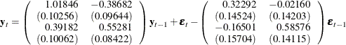
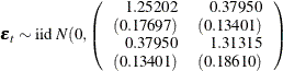
The fitted VARMA(1,1) model with estimated standard errors in parentheses is given as
and
VARMAX Modeling
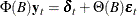
A general VARMAX( ) process is written as
or
where and . The vector  consists of all possible deterministic terms, namely constant, seasonal dummies, linear trend, quadratic trend, and exogenous
variables. The vector
consists of all possible deterministic terms, namely constant, seasonal dummies, linear trend, quadratic trend, and exogenous
variables. The vector  , where
  ;
;  ;
;  , are seasonal dummies and
  is based on the NSEASON= option;
  ; A is the parameter matrix corresponding to
  and
and  for
for  .
.
The state space form of the VARMAX(p,q,s) model consists of a state equation
![\[ \mb{z} _{t} =F\mb{z} _{t-1} + \mb{w}_ t + G\bepsilon _{t} \]](images/etsug_varmax0686.png)
and an observation equation
where
![\[ \mb{z} _{t}=(\mb{y} _{t}’,\mb{y}_{t-1}’,\ldots ,\mb{y} _{t-(v-1)}’, \bepsilon _{t}’, \bepsilon _{t-1},\ldots ,\bepsilon _{t-(q-1)}’, \mb{c}_{t+1}’)’ \]](images/etsug_varmax0687.png)
![\[ F = \left[\begin{matrix} \Phi _{1} & \cdots & \Phi _{v-1} & \Phi _{v} & -\Theta _{1} & \cdots & -\Theta _{q-1} & -\Theta _{q} & \Delta \\ I_ k & \cdots & 0 & 0 & 0 & \cdots & 0 & 0 & 0 \\ \vdots & \ddots & 0 & \vdots & \vdots & \ddots & \vdots & \vdots & \vdots \\ 0 & \cdots & I_ k & 0 & 0 & \cdots & 0 & 0 & 0 \\ 0 & \cdots & 0 & 0 & 0 & \cdots & 0 & 0 & 0 \\ 0 & \cdots & 0 & 0 & I_ k & \cdots & 0 & 0 & 0 \\ \vdots & \ddots & 0 & \vdots & \vdots & \ddots & \vdots & \vdots & \vdots \\ 0 & \cdots & 0 & 0 & 0 & \cdots & I_ k & 0 & 0 \\ \end{matrix} \right], ~ ~ G = \left[\begin{matrix} I_ k \\ 0_{k(v-1) \times k} \\ I_ k \\ 0_{k(q-1) \times k} \\ 0_{ u \times k} \end{matrix}\right] \]](images/etsug_varmax0688.png)
and
![\[ H = [I_ k, 0_{(k(v+q-1)+u) \times k}] \]](images/etsug_varmax0689.png)
where  , for , and u is the dimension of
  .
.
Kalman filtering is used to evaluate the likelihood function. The updating equation is
where
The prediction equation is
![\[ \hat{\mb{z} }_{t|t-1} = F \hat{\mb{z} }_{t-1|t-1} + \mb{w}_ t, ~ ~ P_{t|t-1} = F P_{t-1|t-1} F’ + G \Sigma G’ \]](images/etsug_varmax0692.png)
where for .
The log-likelihood function can be expressed as
where and are determined recursively from Kalman filtering. To construct the likelihood function from Kalman filtering, you obtain
, , and .
In the preceding state space form of a VARMAX model, the exogenous variables are treated as determined terms, which implies that the values of the exogenous variables must be provided to forecast the out-of-sample dependent variables. If you do not have the future values of the exogenous variables, either you predict the exogenous variables in a separate model, or you express both the exogenous variables and the dependent variables in one combined model and predict them together (Reinsel 1997).
The dimension of the state space vector of the Kalman filtering method for the VARMAX(p,q,s) model might be large, so it might take a lot of time and memory for computing.
Two examples of VARMAX modeling follow:
model y1 y2 = x1 / q=1;
nloptions tech=qn;
model y1 y2 = x1 / p=1 q=1 xlag=1 nocurrentx;
nloptions tech=qn;