The VARMAX Procedure

Vector Error Correction Model

Subsections:

Cointegration Testing

A vector error correction model (VECM) can lead to a better understanding of the nature of any nonstationarity among the different component series and can also improve longer-term forecasting compared to an unconstrained model.

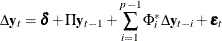
The VECM(p) form with the cointegration rank, $r(\leq k)$ , is written as

$\begin{eqnarray*} \Delta \mb{y} _{t} = \bdelta + \Pi \mb{y} _{t-1} + \sum _{i=1}^{p-1}\Phi ^*_ i \Delta \mb{y} _{t-i} + \bepsilon _ t \end{eqnarray*}$

where $\Delta$ is the differencing operator, such that $\Delta \mb{y} _{t} = \mb{y} _{t}-\mb{y} _{t-1}$ ; $\Pi = \alpha \beta ’$ , where $\alpha$ and $\beta$ are $k\times r$ matrices; and $\Phi ^*_ i$ is a $k\times k$ matrix.

The VECM(p) form has an equivalent VAR(p) representation as described in the section Vector Autoregressive Model.

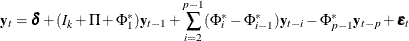
$\begin{eqnarray*} \mb{y} _{t} = \bdelta + (I_ k+\Pi +\Phi ^*_1) \mb{y} _{t-1} +\sum _{i=2}^{p-1} (\Phi ^*_ i-\Phi ^*_{i-1}) \mb{y} _{t-i} -\Phi ^*_{p-1}\mb{y} _{t-p} + \bepsilon _ t \end{eqnarray*}$

where $I_ k$ is a $k\times k$ identity matrix.

An example of the second-order nonstationary vector autoregressive model is

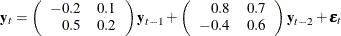
$\begin{eqnarray*} \mb{y} _ t = \left( \begin{array}{rr} -0.2 & 0.1 \\ 0.5 & 0.2 \\ \end{array} \right) \mb{y} _{t-1} + \left( \begin{array}{rr} 0.8 & 0.7 \\ -0.4 & 0.6 \\ \end{array} \right) \mb{y} _{t-2} + \bepsilon _ t \end{eqnarray*}$

with

$\begin{eqnarray*} \Sigma = \left( \begin{array}{rr} 100 & 0 \\ 0 & 100 \\ \end{array} \right) ~ ~ \mr{and} ~ ~ \mb{y} _{-1} = \mb{y} _0 = \left( \begin{array}{r} 0 \\ 0 \\ \end{array} \right) \end{eqnarray*}$

This process can be given the following VECM(2) representation with the cointegration rank one:

$\begin{eqnarray*} \Delta \mb{y} _ t = \left( \begin{array}{r} -0.4 \\ 0.1 \\ \end{array} \right) ( 1, -2 ) \mb{y} _{t-1} - \left( \begin{array}{rr} 0.8 & 0.7 \\ -0.4 & 0.6 \\ \end{array} \right) \Delta \mb{y} _{t-1} + \bepsilon _ t \end{eqnarray*}$

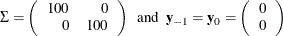
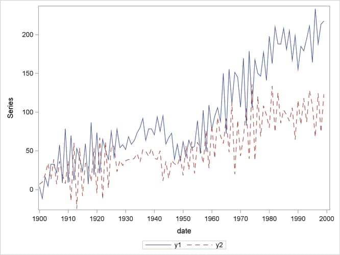
The following PROC IML statements generate simulated data for this VECM(2) form and the PROC SGPLOT statements plot the data, as shown in Figure 42.12:

proc iml;
   sig = 100*i(2);
   phi = {-0.2 0.1, 0.5 0.2, 0.8 0.7, -0.4 0.6};
   call varmasim(y,phi) sigma=sig n=100 initial=0
                        seed=45876;
   cn = {'y1' 'y2'};
   create simul2 from y[colname=cn];
   append from y;
quit;

data simul2;
   set simul2;
   date = intnx( 'year', '01jan1900'd, _n_-1 );
   format date year4. ;
run;

proc sgplot data=simul2;
   series x=date y=y1 / lineattrs=(pattern=solid);
   series x=date y=y2 / lineattrs=(pattern=dash);
   yaxis label="Series";
run;

Figure 42.12: Plot of Generated Data Process

Cointegration Testing

The following statements use the Johansen cointegration rank test. The COINTTEST=(JOHANSEN) option performs the Johansen trace test and is equivalent to specifying the COINTTEST option with no additional suboptions or specifying the COINTTEST=(JOHANSEN=(TYPE=TRACE)) option.

/*--- Cointegration Test ---*/

proc varmax data=simul2;
   model y1 y2 / p=2 noint dftest cointtest=(johansen);
run;

Figure 42.13 shows the output for Dickey-Fuller tests for the nonstationarity of each series and the Johansen cointegration rank test between series.

Figure 42.13: Dickey-Fuller Tests and Cointegration Rank Test

The VARMAX Procedure

Unit Root Test
Variable	Type	Rho	Pr < Rho	Tau	Pr < Tau
y1	Zero Mean	1.47	0.9628	1.65	0.9755
	Single Mean	-0.80	0.9016	-0.47	0.8916
	Trend	-10.88	0.3573	-2.20	0.4815
y2	Zero Mean	-0.05	0.6692	-0.03	0.6707
	Single Mean	-6.03	0.3358	-1.72	0.4204
	Trend	-50.49	0.0003	-4.92	0.0006

Cointegration Rank Test Using Trace
H0: Rank=r	H1: Rank>r	Eigenvalue	Trace	Pr > Trace	Drift in ECM	Drift in Process
0	0	0.5086	70.7279	<.0001	NOINT	Constant
1	1	0.0111	1.0921	0.3441

In Dickey-Fuller tests, the second column specifies three types of models, which are zero mean, single mean, or trend. The third column (Rho) and the fifth column (Tau) are the test statistics that are used to test the null hypothesis that the series has a unit root. Other columns are their p-values. You can see that both series have unit roots. For a description of Dickey-Fuller tests, see the section PROBDF Function for Dickey-Fuller Tests in Chapter 6: SAS Macros and Functions.

In the "Cointegration Rank Test Using Trace" table, the last two columns explain the drift in the model or process. Because the NOINT option is specified, the model is

$\begin{eqnarray*} \Delta \mb{y} _{t} = \Pi \mb{y} _{t-1} + \Phi ^*_1 \Delta \mb{y} _{t-1} + \bepsilon _ t \end{eqnarray*}$

The column Drift in ECM indicates that there is no separate drift in the error correction model, and the column Drift in Process indicates that the process has a constant drift before differencing.

H0 is the null hypothesis, and H1 is the alternative hypothesis. The first row tests the cointegration rank $r=0$ against $r>0$ , and the second row tests $r=1$ against $r>1$ . The trace test statistics in the fourth column are computed by $-T\sum _{i=r+1}^ k \log (1-\lambda _ i)$ , where T is the available number of observations and $\lambda _ i$ is the eigenvalue in the third column. The p-values for these statistics are output in the fifth column. If you compare the p-value in each row to the significance level of interest (such as 5%), the null hypothesis that there is no cointegrated process (H0: $r=0$ ) is rejected, whereas the null hypothesis that there is at most one cointegrated process (H0: $r=1$ ) cannot be rejected.

The following statements fit a VECM(2) form to the simulated data:

/*--- Vector Error Correction Model ---*/

proc varmax data=simul2;
   model y1 y2 / p=2 noint lagmax=3
                 print=(iarr estimates);
   cointeg rank=1 normalize=y1;
run;

The results in Figure 42.13 indicate that the time series are cointegrated with rank = 1. So you might want to specify the RANK=1 option in the COINTEG statement. For normalizing the value of the cointegrated vector, you specify the normalized variable by using the NORMALIZE= option in the COINTEG statement. The COINTEG statement produces the estimates of the long-run parameter, $\bbeta$ , and the adjustment coefficient, $\balpha$ . The PRINT=(IARR) option provides the VAR(2) representation.

The VARMAX procedure output is shown in Figure 42.14 through Figure 42.17. In Figure 42.14, "1" indicates the first column of the $\balpha$ and $\bbeta$ matrices. Because the cointegration rank is 1 in the bivariate system, $\balpha$ and $\bbeta$ are two-dimensional vectors. The estimated cointegrating vector is $\hat{\bbeta }=(1, -1.96)’$ . Therefore, the long-run relationship between $y_{1t}$ and $y_{2t}$ is $y_{1t}=1.96y_{2t}$ . The first element of $\hat{\bbeta }$ is 1 because $y_1$ is specified as the normalized variable. Asymptotically, $\balpha$ follows a normal distribution, and the t values and p-values of its elements are shown in the "Alpha and Beta Parameter Estimates" table; however, because $\bbeta$ follows a nonnormal distribution, the corresponding standard errors, t values, and p-values are missing. The Variable column shows the variables that correspond to the coefficients. For example, for the coefficient $\balpha _{ij}$ (the ith element in the jth column of $\balpha$ ), ALPHA $i\_ j$ , the variable is the inner product of the transpose of the jth column of $\bbeta$ (Beta[,j] $’$ ) and the vector of lag 1 dependent variables $\mb{y} _{t-1}$ ( $\_$ DEP $\_$ (t–1)).

Figure 42.14: Parameter Estimates for the VECM(2) Form

The VARMAX Procedure

Type of Model	VECM(2)
Estimation Method	Maximum Likelihood Estimation
Cointegrated Rank	1

Beta
Variable	1
y1	1.00000
y2	-1.95575

Alpha
Variable	1
y1	-0.46680
y2	0.10667

Alpha and Beta Parameter Estimates
Equation	Parameter	Estimate	Standard Error	t Value	Pr > \|t\|	Variable
D_y1	ALPHA1_1	-0.46680	0.04786	-9.75	<.0001	Beta[,1]'*_DEP_(t-1)
	BETA1_1	1.00000				y1(t-1)
D_y2	ALPHA2_1	0.10667	0.05146	2.07	0.0409	Beta[,1]'*_DEP_(t-1)
	BETA2_1	-1.95575				y2(t-1)

Figure 42.15 shows the parameter estimates in terms of lag 1 coefficients, $\mb{y} _{t-1}$ , and lag 1 first-differenced coefficients, $\Delta \mb{y} _{t-1}$ , and their significance. "Alpha * Beta $’$ " indicates the coefficients of $\mb{y} _{t-1}$ and is obtained by multiplying the Alpha and Beta estimates in Figure 42.14. The parameter AR1 $\_ i\_ j$ (which is shown in the "Model Parameter Estimates" table) corresponds to the elements in the "Alpha * Beta $’$ " matrix. The parameter AR2 $\_ i\_ j$ corresponds to the elements in the differenced lagged AR coefficient matrix. The "D_" prefixed to a variable name in Figure 42.15 implies differencing.

Figure 42.15: Parameter Estimates for the VECM(2) Form, Continued

Parameter Alpha * Beta' Estimates
Variable	y1	y2
y1	-0.46680	0.91295
y2	0.10667	-0.20862

AR Coefficients of Differenced Lag
DIF Lag	Variable	y1	y2
1	y1	-0.74332	-0.74621
	y2	0.40493	-0.57157

Model Parameter Estimates
Equation	Parameter	Estimate	Standard Error	t Value	Pr > \|t\|	Variable
D_y1	AR1_1_1	-0.46680	0.04786	-9.75	<.0001	y1(t-1)
	AR1_1_2	0.91295	0.09359	9.75	<.0001	y2(t-1)
	AR2_1_1	-0.74332	0.04526	-16.42	<.0001	D_y1(t-1)
	AR2_1_2	-0.74621	0.04769	-15.65	<.0001	D_y2(t-1)
D_y2	AR1_2_1	0.10667	0.05146	2.07	0.0409	y1(t-1)
	AR1_2_2	-0.20862	0.10064	-2.07	0.0409	y2(t-1)
	AR2_2_1	0.40493	0.04867	8.32	<.0001	D_y1(t-1)
	AR2_2_2	-0.57157	0.05128	-11.15	<.0001	D_y2(t-1)

Figure 42.16 shows the parameter estimates of the innovations covariance matrix and their significance.

Figure 42.16: Parameter Estimates for the VECM(2) Form, Continued

Covariance Parameter Estimates
Parameter	Estimate	Standard Error	t Value	Pr > \|t\|
COV1_1	94.75575	13.53654	7.00	<.0001
COV1_2	4.52684	10.30302	0.44	0.6614
COV2_2	109.57038	15.65291	7.00	<.0001

The fitted model is represented as

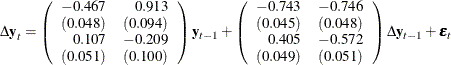
$\begin{eqnarray*} {\Delta \mb{y} }_ t = \left( \begin{array}{rr} -0.467 & 0.913 \\ (0.048) & (0.094)\\ 0.107 & -0.209 \\ (0.051) & (0.100)\\ \end{array} \right) \mb{y} _{t-1} + \left( \begin{array}{rr} -0.743 & -0.746 \\ (0.045)& (0.048) \\ 0.405 & -0.572 \\ (0.049) & (0.051)\\ \end{array} \right) \Delta \mb{y} _{t-1} + \bepsilon _ t \end{eqnarray*}$

Figure 42.17: Change the VECM(2) Form to the VAR(2) Model

Infinite Order AR Representation
Lag	Variable	y1	y2
1	y1	-0.21013	0.16674
	y2	0.51160	0.21980
2	y1	0.74332	0.74621
	y2	-0.40493	0.57157
3	y1	0.00000	0.00000
	y2	0.00000	0.00000

The PRINT=(IARR) option in the previous SAS statements prints the reparameterized coefficient estimates. Because LAGMAX=3 in those statements, the coefficient matrix of lag 3 is zero.

The VECM(2) form in Figure 42.17 can be rewritten as the following second-order vector autoregressive model:

$\begin{eqnarray*} \mb{y} _ t = \left( \begin{array}{rr} -0.210 & 0.167 \\ 0.512 & 0.220 \end{array} \right) \mb{y} _{t-1} + \left( \begin{array}{rr} 0.743 & 0.746 \\ -0.405 & 0.572 \end{array} \right) \mb{y} _{t-2} + \bepsilon _ t \end{eqnarray*}$