The VARMAX Procedure

Parameter Estimation and Testing on Restrictions

In the previous example, the VARX(1,0) model is written as

$\begin{eqnarray*} \mb{y} _{t} = \bdelta + \Theta ^{*}_0\mb{x} _{t} + \Phi _1\mb{y} _{t-1} + \bepsilon _ t \end{eqnarray*}$

with

$\begin{eqnarray*} \Theta _0^{*} = \left( \begin{array}{rr} \theta ^{*}_{11} & \theta ^{*}_{12} \\ \theta ^{*}_{21} & \theta ^{*}_{22} \\ \theta ^{*}_{31} & \theta ^{*}_{32} \end{array} \right) ~ ~ ~ \Phi _1 = \left( \begin{array}{rrr} \phi _{11} & \phi _{12} & \phi _{13} \\ \phi _{21} & \phi _{22} & \phi _{23} \\ \phi _{31} & \phi _{32} & \phi _{33} \end{array} \right) \end{eqnarray*}$

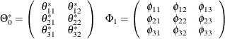
In Figure 42.21 of the preceding section, you can see several insignificant parameters. For example, the coefficients XL0_1_2, AR1_1_2, and AR1_3_2 are insignificant.

The following statements restrict the coefficients of 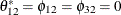$\theta _{12}^*=\phi _{12}=\phi _{32}=0$ for the VARX(1,0) model.

/*--- Models with Restrictions and Tests ---*/

proc varmax data=grunfeld;
   model y1-y3 = x1 x2 / p=1 print=(estimates);
   restrict XL(0,1,2)=0, AR(1,1,2)=0, AR(1,3,2)=0;
run;

The output in Figure 42.22 shows that three parameters $\theta _{12}^*$ , $\phi _{12}$ , and $\phi _{32}$ are replaced by the restricted values, zeros, and their standard errors are also zeros to indicate that the parameters are fixed to these values.

Figure 42.22: Parameter Estimation with Restrictions

The VARMAX Procedure

Model Parameter Estimates
Equation	Parameter	Estimate	Standard Error	t Value	Pr > \|t\|	Variable
y1	CONST1	-2.16781	13.13755	-0.17	0.8715	1
	XL0_1_1	1.67592	0.40792	4.11	0.0012	x1(t)
	XL0_1_2	0.00000	0.00000			x2(t)
	AR1_1_1	0.27671	0.17606	1.57	0.1401	y1(t-1)
	AR1_1_2	0.00000	0.00000			y2(t-1)
	AR1_1_3	0.01747	0.03519	0.50	0.6279	y3(t-1)
y2	CONST2	768.14598	224.12735	3.43	0.0045	1
	XL0_2_1	-6.30880	4.85729	-1.30	0.2166	x1(t)
	XL0_2_2	2.65308	0.43840	6.05	0.0001	x2(t)
	AR1_2_1	-2.16968	1.83550	-1.18	0.2584	y1(t-1)
	AR1_2_2	0.10945	0.11751	0.93	0.3686	y2(t-1)
	AR1_2_3	-0.93053	0.41478	-2.24	0.0429	y3(t-1)
y3	CONST3	-19.88165	7.69575	-2.58	0.0227	1
	XL0_3_1	-0.03576	0.20079	-0.18	0.8614	x1(t)
	XL0_3_2	-0.00919	0.01747	-0.53	0.6076	x2(t)
	AR1_3_1	0.96398	0.06907	13.96	0.0001	y1(t-1)
	AR1_3_2	0.00000	0.00000			y2(t-1)
	AR1_3_3	0.93412	0.01473	63.41	0.0001	y3(t-1)

The output in Figure 42.23 shows the estimates of the Lagrangian parameters and their significance. Based on the p-values associated with the Lagrangian parameters, you cannot reject the null hypotheses $\theta _{12}^*=0$ , $\phi _{12}=0$ , and $\phi _{32}=0$ with the 0.05 significance level.

Figure 42.23: RESTRICT Statement Results

Testing of the Restricted Parameters
Parameter	Estimate	Standard Error	t Value	Pr > \|t\|	Equation
Restrict0	1.74969	21.44026	0.08	0.9389	XL0_1_2 = 0
Restrict1	30.36254	70.74347	0.43	0.6899	AR1_1_2 = 0
Restrict2	55.42191	164.03075	0.34	0.7524	AR1_3_2 = 0

The TEST statement in the following example tests $\phi _{31}=0$ and $\theta _{12}^*=\phi _{12}=\phi _{32}=0$ for the VARX(1,0) model:

proc varmax data=grunfeld;
   model y1-y3 = x1 x2 / p=1;
   test AR(1,3,1)=0;
   test XL(0,1,2)=0, AR(1,1,2)=0, AR(1,3,2)=0;
run;

The output in Figure 42.24 shows that the first column in the output is the index corresponding to each TEST statement. You can reject the hypothesis test $\phi _{31}=0$ at the 0.05 significance level, but you cannot reject the joint hypothesis test $\theta _{12}^*=\phi _{12}=\phi _{32}=0$ at the 0.05 significance level.

Figure 42.24: TEST Statement Results

The VARMAX Procedure

Testing of the Parameters
Test	DF	Chi-Square	Pr > ChiSq
1	1	150.31	<.0001
2	3	0.34	0.9522