The VARMAX Procedure
- Overview
-
Getting Started

-
Syntax
-
DetailsMissing ValuesVARMAX ModelDynamic Simultaneous Equations ModelingImpulse Response FunctionForecastingTentative Order SelectionVAR and VARX ModelingSeasonal Dummies and Time TrendsBayesian VAR and VARX ModelingVARMA and VARMAX ModelingModel Diagnostic ChecksCointegrationVector Error Correction ModelingI(2) ModelVector Error Correction Model in ARMA FormMultivariate GARCH ModelingOutput Data SetsOUT= Data SetOUTEST= Data SetOUTHT= Data SetOUTSTAT= Data SetPrinted OutputODS Table NamesODS GraphicsComputational Issues
-
Examples
- References
I(2) Model
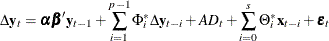
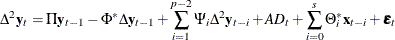
The VARX(p,s) model can be written in the error correction form:
Let  .
.
If  and
and  have full-rank r, and
  , then
  is an
is an  process.
If the condition  fails and
  has reduced-rank
  where
where  and
and  are
are  matrices with
  , then
  and
and  are defined as
  matrices of full rank such that
  and
and  .
.
If and have full-rank s, then the process  is
is  , which has the implication of model for the moving-average representation.
The matrices  ,
,  , and
, and  are determined by the cointegration properties of the process, and
  and
and  are determined by the initial values. For details, see Johansen (1995b).
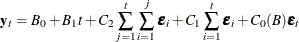
The implication of the model for the autoregressive representation is given by
where  and .
and .
Test for I(2)
The cointegrated model is given by the following parameter restrictions:

where and are matrices with  . Let
. Let  represent the model where and have full-rank r, let
  represent the model where and have full-rank s, and let
  represent the model where and have rank
  . The following table shows the relation between the models and the models.
Table 42.6: Relation between the and Models
|
|
|
||||||||||
|
|
k |
|
|
1 |
|||||||
|
0 |
|
|
|
|
|
|
|
|
|
= |
|
|
1 |
|
|
|
|
|
|
|
= |
|
||
|
|
|
|
|
|
|
||||||
|
|
|
|
|
= |
|


Johansen (1995b) proposed the two-step procedure to analyze the model. In the first step, the values of  are estimated using the reduced rank regression analysis, performing the regression analysis
  ,
,  , and
, and  on
on 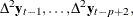 and
and  . This gives residuals
  ,
,  , and
, and  , and residual product moment matrices
![\[ M_{ij} = \frac{1}{T} \sum _{t=1}^ TR_{it}R_{jt}’ ~ ~ \mr{for~ ~ } i,j=0,1,2 \]](images/etsug_varmax0986.png)
Perform the reduced rank regression analysis on corrected for , and , and solve the eigenvalue problem of the equation
![\[ |\lambda M_{22\mb{.} 1} - M_{20\mb{.} 1}M_{00\mb{.} 1}^{-1}M_{02\mb{.} 1}| = 0 \]](images/etsug_varmax0987.png)
where 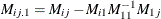 for
for  .
.
In the second step, if are known, the values of  are determined using the reduced rank regression analysis, regressing
  on
on  corrected for
  , and
, and  .
.
The reduced rank regression analysis reduces to the solution of an eigenvalue problem for the equation

where
where  .
.
The solution gives eigenvalues 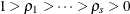 and eigenvectors
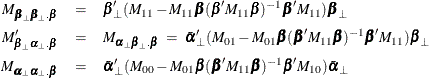
  . Then, the ML estimators are
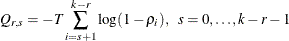
The likelihood ratio test for the reduced rank model with rank in the model  is given by
The following statements simulate an I(2) process and compute the rank test to test for cointegrated order 2:
proc iml;
   alpha  = { 1, 1};    * alphaOrthogonal = { 1, -1};
   beta   = { 1, -0.5}; * betaOrthogonal  = { 1, 2};
   * alphaOrthogonal' * phiStar * betaOrthogonal = 0;
   phiStar = { 1 0, 0 0.5};
   A1 = 2 * I(2) + alpha * beta` - phiStar;
   A2 = phiStar - I(2);
   phi = A1 // A2;
   sig = I(2);
   /* to simulate the vector time series */
   call varmasim(y,phi) sigma=sig n=200 seed=2;
   cn = {'y1' 'y2'};
   create simul4 from y[colname=cn];
   append from y;
   close;
quit;

proc varmax data=simul4;
   model y1 y2 /noint p=2 cointtest=(johansen=(iorder=2));
run;
The last two columns in Figure 42.76 explain the cointegration rank test with integrated order 1. For a specified significance level, such as 5%, the output indicates
that the null hypothesis that the series are not cointegrated (H0:  ) is rejected, because the p-value for this test, shown in the column Pr > Trace of I(1), is less than 0.05. The results also indicate that the null hypothesis
that there is a cointegrated relationship with cointegration rank 1 (H0:
) is rejected, because the p-value for this test, shown in the column Pr > Trace of I(1), is less than 0.05. The results also indicate that the null hypothesis
that there is a cointegrated relationship with cointegration rank 1 (H0:  ) cannot be rejected at the 5% significance level, because the p-value for the test statistic, 0.7961, is greater than 0.05. Because of this latter result, the rows in the table that are
associated with are further examined. The test statistic, 0.0257, tests the null hypothesis that the series are cointegrated order 2. The
p-value that is associated with this test is 0.8955, which indicates that the null hypothesis cannot be rejected at the 5%
significance level.
) cannot be rejected at the 5% significance level, because the p-value for the test statistic, 0.7961, is greater than 0.05. Because of this latter result, the rows in the table that are
associated with are further examined. The test statistic, 0.0257, tests the null hypothesis that the series are cointegrated order 2. The
p-value that is associated with this test is 0.8955, which indicates that the null hypothesis cannot be rejected at the 5%
significance level.
Figure 42.76: Cointegrated I(2) Test (IORDER= Option)